Lately, the excitement around quantum computing has reached our database community, and it raises a natural question: Can quantum computing help our database systems? The real answer is more modest than the hype suggests, but also more concrete than the skeptics assume. In this post, I try to pin down exactly where it is real.

First, what quantum is good at for databases

Database systems perform many different kinds of work, but quantum computing is not equally suited to all of them. Its clearest potential lies in optimization problems where a small input gives rise to an enormous number of possible solutions. Join ordering, index selection, workload optimization, and transaction scheduling all have this shape. To understand why quantum computing may help with these problems, we first need a brief look at what makes it different from classical computing.

A classical computer stores bits, and each bit is either a 0 or a 1. A quantum computer instead stores qubits, and a qubit can hold a blend of 0 and 1 at the same time. A coin is a good way to picture this. A classical bit is a coin lying flat, showing heads or tails. A qubit is a coin spinning in the air, in a blend of both at once, and it becomes definitely heads or tails only when it lands, which is the moment we measure it. That spinning blend is called superposition. Qubits can also be linked, so that measuring one instantly tells you something about another. This property is called entanglement, and even Einstein found it spooky. Together, these two properties allow quantum algorithms to explore large spaces of possible solutions in ways that classical bits cannot. With n classical bits, you can store exactly one of the 2^n possible patterns at any instant. With n qubits, you can hold a weighted blend of all 2^n at once, and entanglement lets those possibilities interfere and reinforce one another. A quantum algorithm is designed so that paths leading to wrong answers cancel out, while paths leading to right answers reinforce. The correct result is then far more likely to appear when we finally measure. There is a catch, though. Qubits are fragile. They lose their delicate state to heat, stray fields, and other noise, an effect called decoherence, and every operation adds a little error. On today’s hardware, these errors pile up quickly, which is why a real quantum computer is far less reliable than the clean picture above. 

Two algorithms, both introduced a few decades ago, are responsible for most of the excitement about quantum computing. Grover’s search [1] looks for a marked item in a completely unstructured space of N candidates. It finds that item in about the square root of N tries, a quadratic speedup over the roughly N tries a classical scan needs in the worst case. Despite its name and its superficial resemblance to database search, Grover’s algorithm does not mean that a quantum computer can simply replace a database index or accelerate an ordinary table scan. Loading database records into a quantum device and retrieving the result introduce fundamental practical limitations. Shor’s algorithm [2] factors a large integer in time that grows only polynomially with the number’s size. That is exponentially faster than the best classical methods we know, and it is what threatens the RSA-style encryption that protects your bank details. Both algorithms are backed by real mathematics. However, both also assume a large-scale, reliable, error-corrected quantum computer that does not quite exist yet.

But you do not need a full universal quantum computer to attack an optimization problem. Two nearer-term styles do exactly that. “Quantum annealing” takes a hard optimization problem with many discrete choices and encodes it as an energy landscape. The hardware then settles into a low valley that corresponds to a good, near-optimal solution. One phenomenon of quantum annealing is worth knowing here: quantum tunneling. A classical search, like simulated annealing, has to climb over a tall hill to escape a bad solution. A quantum system can pass straight through the hill instead, slipping out of the local traps that stall ordinary methods. “Variational methods”, such as QAOA, take a different route. They run a small, tunable quantum circuit on a gate-based device, while a classical optimizer adjusts its knobs round after round toward a good solution. These two paradigms differ in how easily they fit inside a real-time system today. A quantum annealer returns many candidate solutions in a single quick call, which suits tight time budgets. A variational method needs many circuit runs inside a classical optimization loop, so it is more flexible but, for now, slower to drop into a live query engine. When you read “quantum for databases” these days, it almost always means annealing or variational methods, not the far-off universal gate-based dream. That is no accident: databases are full of hard combinatorial optimization problems, which is exactly what these methods target. As error correction matures, general gate-based computing may bring a wider range of database problems within reach. For now, though, hybrid classical-quantum optimization is where the practical work happens.

The best way to think about exploiting quantum computing in a database system today is as an “accelerator,” similar to today’s CPU-GPU computation model. There, the CPU stays in charge and offloads its most compute-heavy, data-parallel kernels to a GPU that is built for exactly that kind of work. A quantum optimizer can play the same role for a database engine, taking on hard optimization sub-problems while the classical engine runs everything else. Now, let’s look at where this accelerator genuinely helps, and then turn to where it does not.

What is real

Quantum machines are bad at taking in large amounts of data, but many of our hardest database optimization problems are not about large data at all. They start from a small input and blow up into a huge search space. Join order optimization is the standard example: the input consists of just a few tables and some statistics, yet the number of possible plans grows exponentially as tables are added. Reusing shared work across many queries, picking a set of indexes under a storage budget, and scheduling transactions all look the same way: a small input with an enormous number of ways to arrange it. This is exactly the shape quantum optimization is built for. But the device cannot read a query plan directly, so you first represent the problem in a form the hardware understands. For example, with annealers, that form is called QUBO, short for Quadratic Unconstrained Binary Optimization. Each decision becomes a 0/1 variable, and the cost you want to minimize becomes a sum of penalties over those variables and their pairs (i.e., correlations). A low-cost setting of the variables then corresponds to a good plan. Variational methods encode the same kind of objective for gate-based hardware.

Importantly, this line of research has progressed from problem formulations and isolated evaluations toward real-hardware integration. Earlier work mapped multiple-query optimization to a formulation suitable for D-Wave annealers [5], while subsequent studies explored quantum approaches to query optimization and transaction scheduling more broadly [6]. Today, a D-Wave annealer with more than 5,000 qubits is accessible through the cloud, so hardware access is no longer the main obstacle. The harder question is whether the gains survive after the method is integrated into a real engine and all overhead is counted. The QDBO prototype [3] takes a step in this direction by integrating a quantum-augmented optimizer directly with PostgreSQL. It casts each optimization task into QUBO form and refines the answer using the annealer’s sampling feedback. As one example, on the Cardinality Estimation Benchmark, QDBO achieved up to 49 times execution-time speedup and up to 37 times end-to-end speedup, including quantum and cloud overhead. These results simply show that “faster end to end, inside a real engine, on real hardware” is now something we can actually achieve.

What is still hard

The quantum-based results are promising, but they remain demonstrations rather than large-scale deployments. Turning a working demo into a production system means addressing problems that the excitement usually skips over. Here, I lay out three challenges that keep coming up when we put quantum computing to work inside database systems. What strikes me about all three is that they are database problems more than quantum-hardware problems. 

The first is controlling the hybrid classical-quantum workflow. The easy approach to performing quantum optimization is to use a hosted, black-box quantum solver (e.g., D-Wave’s Stride or Amazon’s Braket). You hand over the optimization problem and get an answer back, with no view into what the service does internally, how long it runs on the quantum processor (QPU), or how it arrives at the final answer. Some services even enforce a minimum response time of several seconds, which is a non-starter for a query planner that has milliseconds to spend. The alternative is to run the loop yourself, choosing how to sample and how to spend a time budget you can adjust on the fly. QDBO [3] demonstrated that, by driving the quantum sampling directly, you can outperform the vendor’s black-box solver and stay within a real latency budget. However, this work only scratched the surface, and a general way to trade solution quality for time across many kinds of queries is still missing. Transparency here is not good manners; it is the performance lever.

The second is scalability, which really turns out to be a consistency problem. For example, a 50-relation join already needs more than 10,000 optimization variables to be mapped to qubits, while the largest annealer offers only about 5,000 qubits, still far more than gate-based models provide. So the whole problem will not fit on the machine at once. You have to break it into smaller sub-problems that do fit, solve each one, and stitch the answers back together. The final quality then depends less on solving each piece well than on how carefully you handle the boundaries where the pieces meet. Getting that global consistency right, rather than just optimizing fragments, is an open problem. It is one that databases have long experience with.

The third is data management, which is where our field’s instincts help most directly. A single quantum run produces information worth keeping: how a large problem was broken up, which optimization variable was mapped to which qubit, and the partial results that came back. Today, all of that is thrown away between runs. Treated instead like reusable materialized views or caches, that information could be maintained, looked up, and reused whenever a later problem overlaps with an earlier one. The optimizer could then skip work it has already done, and the scheduler could load a prepared mapping instead of rebuilding it. Intermediate quantum-workflow data deserves real storage management, not a temporary file.

Underneath all three challenges sits one blunt measurement, and it is why I keep calling this an integration problem rather than a hardware one. In one of our query-optimization runs [4], a single call to the quantum optimizer took about 3,200 milliseconds end to end, from the database sending the problem to getting a plan back. Of that time, the quantum processor itself was busy for well under 100 milliseconds. Almost all the rest went to cloud communication and classical solving. The quantum device is not the bottleneck. The round trips and orchestration around it are, and those are ours to fix.

The quantum hardware is not standing still either. Two advances now taking shape will widen what quantum can reach for databases, and both are worth watching today, not in ten years. The first is “quantum error correction”, which bundles many noisy physical qubits into a single, more reliable one. Recent hardware milestones suggest the field is turning the corner. As reliable qubits arrive, the fragile gate-based machines become real candidates, and the range of database problems quantum computing can touch grows well beyond annealing-friendly optimization. The second is “distributed quantum computing”, which links several processors into one larger fabric, much as we once networked classical machines. It would lift the qubit ceiling that limits problem size today and bring larger join graphs and workload-wide index tuning into range. Neither is here at full strength nowadays, but both are close enough to plan for.

The other direction, briefly

So far, I have focused on quantum for databases. There are also research opportunities in the reverse direction, databases for quantum. Because large error-corrected machines do not yet exist, we rely on classical computers to simulate and prepare quantum circuits, and it turns out that database techniques can help. Mapping quantum states and operations onto relational queries, and using query processing to drive circuit simulation and transpilation, are real and useful ideas [7]. Earlier work also explored representing relational data and relational operations in quantum form [8], although measurement remains a deep obstacle because reading a quantum state changes it. This direction is genuinely interesting, and I invite our community to explore it. 

Open questions

Let me end with a few questions that are still open, the ones I encourage our community to help answer.

Where does quantum genuinely help data management beyond join ordering? Optimization is the beachhead. Is there a second one, perhaps privacy primitives with no classical analogue, or sampling for approximate query processing, that clears the same end-to-end bar?

Which database problems are honestly poor matches? Anything that needs large concrete data loaded into the device seems disqualified. What else belongs on the “do not bother” list, and can we agree on it so that students stop rediscovering it the hard way?

What should a fair benchmark measure? If a better formulation score is the wrong metric and end-to-end latency in a real DBMS is the right one, then who builds the shared benchmark that lets us compare quantum, classical, and learned methods on equal footing?

Which of our own methods could help the quantum side? Cost-based optimization, materialized views, adaptive query processing? How many of these transfer directly to orchestrating quantum workloads?

My bet is that the next real progress here will not come from waiting for a quantum machine that makes integration unnecessary. It will come from database people treating the quantum processor as one more accelerator to integrate well, the way we once learned to use any hardware accelerator (e.g., GPUs, TPUs). If that is right, the work in front of us is familiar work.

References

[1] Lov K. Grover. “A fast quantum mechanical algorithm for database search.” In Proceedings of the 28th Annual ACM Symposium on Theory of Computing (STOC ’96), pages 212-219, 1996.

[2] Peter W. Shor. “Polynomial-Time Algorithms for Prime Factorization and Discrete Logarithms on a Quantum Computer.” SIAM Journal on Computing, 26(5):1484-1509, 1997. (Earlier version in Proceedings of the 35th Annual Symposium on Foundations of Computer Science (FOCS), 1994.)

[3] Hanwen Liu, Abhishek Kumar, Federico Spedalieri, and Ibrahim Sabek. “QDBO: A Real-time Quantum-augmented Database System Optimizer.” Proceedings of the VLDB Endowment (PVLDB), 19(11):3606-3620, 2026.

[4] Hanwen Liu and Ibrahim Sabek. “Towards a Hybrid Quantum-Classical Computing Framework for Database Optimization Problems in a Real-Time Setup.” In Proceedings of the IEEE International Conference on Data Engineering (ICDE), 2026.

[5] Immanuel Trummer and Christoph Koch. “Multiple Query Optimization on the D-Wave 2X Adiabatic Quantum Computer.” Proceedings of the VLDB Endowment (PVLDB), 9(9):648-659, 2016.

[6] Umut Çalikyilmaz, Sven Groppe, Jinghua Groppe, Tobias Winker, Stefan Prestel, Farida Shagieva, Daanish Arya, Florian Preis, and Le Gruenwald. “Opportunities for Quantum Acceleration of Databases: Optimization of Queries and Transaction Schedules.” Proceedings of the VLDB Endowment (PVLDB), 16(9):2344-2353, 2023.

[7] Andrei Ilinescu, Aadi Patwardhan, and Rihan Hai. “InferQ: A Database-Oriented Benchmark for Quantum Circuits Simulation.” Proceedings of the ACM on Management of Data (SIGMOD), 4(4), 2026.

[8] Paul Cockshott. “Quantum Relational Databases.” arXiv:quant-ph/9712025, 1997.

Author Bio: Ibrahim Sabek is an Assistant Professor of Computer Science at the University of Southern California. He leads the Next-generation Data-Intensive Systems Group (NexDIG), where his research focuses on building the next generation of data management, processing, and analysis systems using quantum computing and machine learning. Before joining USC, Ibrahim was a Postdoctoral Associate with the MIT Data Systems Group. He earned his PhD in Computer Science from the University of Minnesota. His research has been recognized with several awards and honors, including the 2026 NSF CAREER Award, the 2025 Google ML and Systems Junior Faculty Award, the 2024 and 2025 Google Data Analytics and Insights (DANI) Awards, and the NSF Computing Innovation Fellowship (2020-2023), among others. For more information, please visit his website: https://viterbi-web.usc.edu/~sabek/.

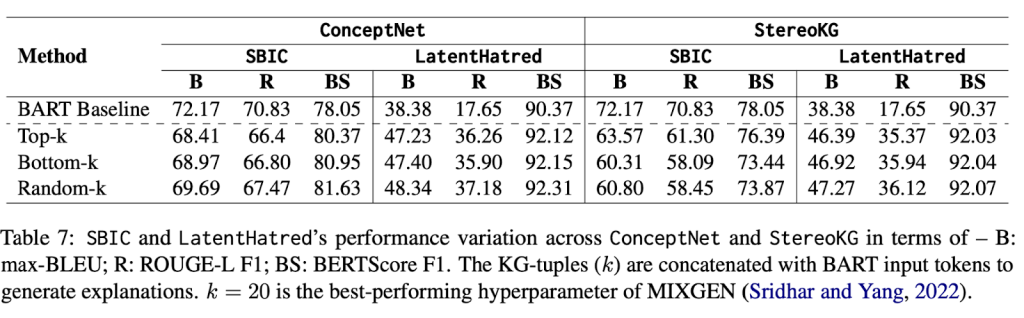
Setup: Using the task of implicit hate explanation, where, for a given implicit hate speech, the aim is to generate a short text explaining the implied context matching the manual/golden explanation, we test the above hypothesis.

We incorporated two implicit hate explanation datasets of varying sizes, and two KGs of different specificity (one general purpose and one task-oriented). We finetuned variants of the BART-base language model to observe changes in knowledge infusion at the input stage (i.e concatenation of knowledge tuples with input hate speech). The change was recorded in terms of natural language generation (NLG) performance metrics, which are the de facto standard for reporting on any generative task. In total, for a given dataset, we obtained four finetuned models per KG. k=20 is adopted from existing literature in hate explanation [2].

Initial observations: Overall, we observed that compared with the base case (no external knowledge infusion), the addition of top-k KG tuples led to a performance increase in one dataset and degradation in another (Table 7). More interesting was the fact that comparing top-k, bottom-k, and random-k in any of the datasets+KG setups did not display any visible degradation in performance. Significance testing with the dataset that initially benefited from top-k further indicated that, by chance, replacing top-k tuples with random-k or bottom-k will not significantly alter the metric-level performance (Table 8).

Manual inspection: To ascertain the low quality of KG tuples, we manually inspected randomly selected 20 samples from each dataset+KG pair. We clearly observed that the top-k tuples showcased that very few contain task-specific, i.e., very few were successful in conveying a hateful connotation. Since the standard process of TF-IDF or cosine similarity-based query-KG matching, as well as ranking, is task agnostic in general, the tuples so obtained are also task agnostic and less diverse. The low diversity of tuples was also quantified by observing the distribution of relevance scores (employed to rank the tuples for the top-k filter) for the dataset+KG pair. 

For detailed results, we encourage readers to check out Section 5 of our paper [3]. 

Some potential solutions: Some clear takeaways emerging from our endeavour are:

1. Generic retrieval techniques, while scalable, come at the cost of task-specific performance. Whether the task-specific approach is to be introduced in the querying step or the ranking step remains an open question. Both come with their pros and cons. I postulate that performing better filtering at the query level would be more effective (trickle-down effect). For example, for toxicity explanation, if we can determine which spans of text are indicators of the vulnerable group being targeted, then those spans can receive a higher weightage when the query vector is generated.  
2.  Secondly, the evaluation of knowledge infusion, especially KG-tuples, needs to accommodate task-specific metrics. For example, in our task, the assessment can be the increase in explicit toxicity when the implied explanations are KG-infused vs not [3].  Such metrics can also be used as a reward for the loss function during finetuning. 
3. Lastly, our experiment reveals that human evaluations are critical even if done on a small scale. Employing LLMs-as-judge to augment human evaluations at scale can be one way forward.

Open questions for the research community: 

In addition to our potential solutions, there remain some broad, open questions for knowledge infusion:

1. Firstly, for heterogeneous knowledge graphs, how can we better incorporate the topology (non-sequential structure) in seq-2-seq models? 
2. Our experiments were run on BART, but at what size of language models, especially for large language models (LLMs), does RAG-based knowledge infusion become ineffective? [4]
3. Our work [3] and previous work [2] in toxicity explanations have found that infusing external context works better at the input level compared to late fusion. However, in the case of explaining memes, late fusion seems to work better [7]. How different NLP tasks behave w.r.t fusion techniques is an interesting question that can help reduce the search space of experiments to run w.r.t knowledge infusion.
4. For knowledge graphs, how can we better incorporate multi-hop connections? Moreover, at what hop should the retrieval stop? Can some task-specific thresholding be employed?

References:

1. Sharma. Retrieval-Augmented Generation: A Comprehensive Survey of Architectures, Enhancements, and Robustness Frontiers. In arxiv. 2025.
2. Shridhar & Yang. Explaining Toxic Text via Knowledge Enhanced Text Generation. In NAACL. 2022.
3. Masud, et al. Tox-BART: Leveraging Toxicity Attributes for Explanation Generation of Implicit Hate Speech. In ACL Findings. 2024.
4. Fayyaz, et al. Collapse of Dense Retrievers: Short, Early, and Literal Biases Outranking Factual Evidence. In ACL. 2025.
5. Shivam, et al. MEMEX: Detecting Explanatory Evidence for Memes via Knowledge-Enriched Contextualization. In ACL. 2023.
6. Shivani, et al. When did you become so smart, oh wise one?! Sarcasm Explanation in Multi-modal Multi-party Dialogues. In ACL. 2022.
7. Abdullakutty & Naseem. Decoding Memes: A Comprehensive Analysis of Late and Early Fusion Models for Explainable Meme Analysis. In WWW Companion Proceedings. 2024.

Author Bio: Sarah Masud is currently a postdoc at the University of Copenhagen, exploring stereotypes and narratives. During her PhD from Indraprastha Institute of Information Technology, New Delhi, she explored the role of different context cues in improving computational hate speech-related tasks. One such work led her to study how knowledge graph tuples impact the generation of toxicity-explaining text. More about her work can be found here: https://sara-02.github.io/ 

Organizers: Eugene Wu, Raul Castro Fernandez 

Panelists: 

• Dan Suciu: Microsoft Endowed Professor in CSE at the University of Washington.
• Sihem Amer-Yahia: Research Director, CNRS, LIG; VP of VLDB Endowment.
• Yannis Ioannidis: Professor of Informatics & Telecom at the University of Athens, President of the ACM.
• Ippokratis Pandis: Distinguished Engineer at Databricks.
• Jens Dittrich, Professor of CS at Saarland University; 3x CIDR gong show winner.

Overview

As organizers, we aimed to foster a bottom-up discussion on the evolving role and future direction of academic database research. Motivated by seismic technological and budgetary shifts, particularly the rise of AI, we explored the comparative advantage of the academic database community. This advantage is critical because it dictates our ability to recruit top students, ensure their success after graduation, and maintain our relevance in a rapidly changing technology and economic landscape. We specifically emphasized that “we” refers to academic database research, contextualizing the topic around recent shifts in government funding ($4B NSF expected budget for 2026) compared to the rapid growth of private investment in AI (e.g., >$100B VC funding in 2024, >$50B in Q1 2025), as funding directly influences the talent landscape.

The feedback for the panel and its structure was as varied as the recommendations themselves. Many approached us afterward to share their excitement in the panel’s discourse and for surfacing their worries and challenges. Others felt the existence of such a panel was yet another in a “sorry tradition of needless negativity” for a vibrant and thriving research community.   With a community as big as ours, we are grateful to receive these diverse opinions.

Matthew Butrovich and Lampros Flokas kindly took notes.  The quoted text below is pulled from these notes, so we do not attribute them to specific individuals.   The post ends with reflections from the organizers.

If this topic is of interest to you, we will be running a companion panel at VLDB 2025 with a different set of panelists, including Shreya Shankar, Gustavo Alonso, Natacha Crooks, Jiannan Wang, and Divesh Srivastava!    We have updated the ArXiv paper to reflect this summary and the panelists’ takes.    Comments and hot takes that you would like to include in the paper are welcome at ewu@cs.columbia.edu and raulcf@uchicago.edu.

Panel Summary

The discussion revolved around two primary topics: the competitive advantage of the academic database research community and actionable strategies for its future.

Our Competitive Advantage

The first topic focused on the academic database community’s competitive advantage as compared to other disciplines, industry, and startups.

Data Principles and AI: Our community’s core database principles, such as “independence between physical and logical” and “declarativeness”, and “automatic scalability hold lasting value. The CTO of Alibaba Cloud demonstrated this by applying query optimization principles to rebuild their pipeline for training QWEN 3, significantly reducing costs. We believe “all AI problems boil to data,” and our deep systems knowledge offers unique insights into challenges like data provenance, security, and novel data abstractions for AI workloads. A panelist noted the “bug” of companies needing hundreds of engineers for each of their separate “AI stack” and “data stack” teams, highlighting a significant opportunity for unified solutions rooted in database thinking.

While some external communities might prioritize immediate problem-solving and “accuracy” over these foundational principles, WE must effectively communicate their long-term benefits. “The way we interact with other communities is problematic” and “we don’t communicate what we have in the right away.”

Navigating the Modern Data Landscape Beyond the Traditional DBMS: “DBMSes are fast enough” for most applications, and our community’s expertise is vital for new data problems beyond the classic RDBMS. For instance, many performance problems are due to the ORM and never arise at the DBMS, while societal-level issues like fake news with an ongoing wave of AI-generated content (“AI slop”) is an information integrity problem. A panelist pointed out that a MacBook can comfortably run TPC-H scale factor 1000: “small data” is enough for most applications and challenges lie in programmability, interoperability, and usability. Conversely, an audience member argued that improving the performance of RDBMSes can also be valuable as throughput increases may unlock new types of applications.

In the AI world, “solutions are crappy when you” combine diverse workloads like vectors, keywords, and relational queries in commercial systems. The platform for building data management systems is “radically different” at “cloud scale,” involving “smart NICs, disaggregated memory that comes and goes, [and] GPU spending.” These new hardware environments present unique opportunities for our deep systems knowledge.

Academic Research Identity: Balancing Curiosity, Impact, and Resources: Academia holds a unique position to pursue “curiosity driven research,” which contrasts with industry’s often shorter-term, product-focused cycles. This allows for “academic play” that breaks free from the need to make numbers go up. Panelists observed that “industry thinks 3/4 quarters ahead” while “Academia thinks 5 years ahead.” Despite industry’s “muscle” (e.g., 600 people on projects compared to “2 students for 2 years” in academia), academia retains the freedom to explore complex, foundational questions without immediate commercial constraints. This implies that academia should not directly compete with industry; as Surajit mentioned in the Tuesday panel, researchers should look for high upside when choosing a problem.

What the Academic Community Should Do

The second half of the panel shifted towards actionable take-aways for the community.

Bring the Data (Researcher) To the Problem: “The way we interact with other communities is problematic” and we expect other communities to come to us. Instead, 1/3 of research sessions in other conferences have ‘data’ in their titles and “these communities are not going to come to SIGMOD”. A key recommendation was to proactively engage with other academic disciplines. The panel stressed the need to “go out” to these communities, and that “inter-disciplinary research post tenure” could be “tremendously fulfilling”. One suggestion was to create “Data + X” workshops in the X communities that are run in a “true discussion mode not as a paper presentation”.

Win the Heart of Data Stakeholders: Despite the lasting value our core database principles, such as “independence between physical and logical” and “declarativeness,” hold, we should not waste our efforts convincing other CS disciplines that these matter. We should direct our efforts toward winning the hearts of data stakeholders. How do we do that? By showing how good we are at treating everything as data and building the data backbone of their needs.  

Improve Dissemination and Communication: There was a strong call to make academic research more accessible and understandable, as “nobody reads our papers, but they want to talk to someone who reads our papers”. It was suggested that papers are “extremely hard to read,” and the community “let[s] others pull the knowledge”. Recommendations included writing “better tutorials” and producing “YouTube videos”, and reducing SIGMOD papers to “8 pages” accompanied by “a clean and fun youtube video”.

Foster Industry-Academia Collaboration: Encouraging students to spend time in industry was highlighted as a way to expose academic research to real-world challenges and bring practical problems back. It was noted that “OpenAI doesn’t come here, but they bought a database” company, Rockset. Their “head of engineering is from Almaden. Send students into industry for a bit after teaching them systems.”

Rethink Conferences and Publication Norms: The panel discussed the need to innovate scholarly communication and conference formats. SIGMOD is a leader in pushing scholarly communication forward (e.g., we introduced reproducibility efforts), and there are ongoing discussions at the SIGMOD and ACM levels about reorganizing conference formats to better support “conferring” over listening to “canned presentations”.   Continuing the idea of academic play, a panelist remarked that our reviewing process may over-index on work that must be faster than some baseline, and inadvertently prune the early seeds of ideas that may not lead to impressive results now but open up impactful research directions in the long run.

Strategically Focus on Foundational Principles in New Contexts: Panelists argued that we need not “become experts in LLMs” or other domains. Instead, our strength lies in forming “multi-disciplinary teams” where each contributes their core expertise. Specifically, for AI, “LLMs are a race to 0. It’s a tool.” Instead, “the application and the data is interesting and where the money is”. The community’s advantage lies in knowing “complexities of modern technology like GPUs” and continually learning.

Closing Comments

The panelists were asked to imagine they were “president of database research” and could unilaterally force one change.

• “Go out and create workshops that are ‘data + X’ or ‘data 4 X’, have them run in a true discussion mode not as a paper presentation with two questions. Interactive panels and a few keynotes by experts. Run interdisciplinary workshops and everyone is forced to go to at least one of them”
• “Force everybody to send students to industry for a bit and bring problems back. security, provenance, data integration. Force a change of mind that academia is the holy land and let students be more open to industry.”
• “Impose that SIGMOD papers be reduced to 8 pages. accompanied by a clean and fun youtube video.”
• “Help people build real applications and make it open source.”

Reflections From the Organizers

Overall, we came away from the panel excited that our community has so much impact, and possesses the data-centric tools that the world needs!    However, our future impact hinges on proactively engaging with a rapidly evolving landscape of applications, evangelizing our expertise to other communities, and strategically collaborating across domains.   All great motivations for academic research!

The positive and insightful discussion ultimately led to recommendations that exhibit inherent trade-offs, rather than a single, clear set of recommendations:

• Is Database Research Art?  We should leverage academia’s unique capacity to pursue curiosity-driven research (academic play), but a real and present budget crisis exists. How do we balance these two imperatives? How can academic research secure sustainable funding for foundational, long-term problems that industry cannot or will not pursue, without becoming irrelevant to the capitalist marketplace that attracts top talent and resources?   It reminds us of artists that strive to pursue purity in expression but face economic realities.
• Impactful Research vs. Market Dominance: We should do impactful research that is neither too short-term nor too long-term, yet offers high upside. However, the relational database market completely dwarfs any alternative data applications and domains. How do we balance the dominance of existing database technologies with the need to explore new paradigms that may not have immediate commercial application but might offer long-term, high-upside impact?
• Go Big and Stay Real: We should talk to other domains and experts to be “trans-disciplinary.” But how do we initiate such projects effectively? What specific models for “multi-disciplinary teams” can integrate deep database knowledge into diverse fields (e.g., AI, quantum computing, social sciences) to solve “data problems” without sacrificing the rigor and identity of database research?
• Engineering vs Science: We encourage students to engage with industry to gain real-world experience, but we also aim to conduct long-term, ambitious scientific research. How do we ensure that industry exposure enriches, rather than detracts from, fundamental scientific inquiry? On the other hand, data management is an applied field, so does it matter?

In either case, we do feel that problems should be paired with solutions. We plan to re-structure the upcoming panel at VLDB 2025 in late August to delve deeper into concrete trade-offs in the above recommendations. If you have suggestions on how to organize the VLDB panel, or would like to share your take on the topic or panel discussion, please share them with ewu@cs.columbia.edu and raulcf@uchicago.edu.

We again thank the panelists, the audience members, people that shared feedback, and Matt Butrovich and Lampros Flokas for taking notes.

The invited experts are Sihem Amer-Yahia (CNRS, Université Grenoble Alpes), Leilani Battle (University of Washington), Yifan Hu (Northeastern University), Dominik Moritz (Carnegie Mellon University & Apple) and Aditya Parameswaran (Berkeley University). This post presents their responses: 

1.Truly Personalized Visual Data Exploration  

Sihem Amer-Yahia, CNRS, Université Grenoble Alpes, France 

Future Challenges 

A visualization is a pair of the form (data, visual element). For instance, data could be a distribution of gender values and the visual element could be a pie chart. A distribution could be mapped to various elements using algebras such as Vega-Lite [1]. Different users appreciate different such mappings. It is hence only natural to ask the question: What is the meaning of personalized data visualization when both data and mapping of data to visual elements can be personalized? Should they both be personalized? Usually, only data is personalized. A follow up question is: Can we learn those visualizations from observing people interacting with data and visual elements? How expressive should this interaction be? How granular should it be? Should we decouple data recommendations from visual recommendations and allow people to provide feedback on them separately and together? Can we do that in a privacy-preserving manner? Finally, since we are talking about users interacting with data and visualizations, how to ensure sub-second interaction time in personalized visual exploration? 

These challenges lay the ground for new research that is truly at the crossroad of databases for privacy-preserving machine learning and declarative visualization. A promising avenue to address all three challenges is to combine the relational algebra with Vega-Lite to extend it to handle in-database Multi-Armed Bandits for online learning [2] and use in-database federated learning to ensure privacy [3]. The augmented algebra will provide the ability to blend data and visualization recommendations in the same framework. It will open new opportunities to co-optimize the training and inference of ML models while taking into consideration user feedback. This is possible by revisiting the reward according to the data and visual elements that are best preferred by the user as they explore (data, visual element) pairs in sequence. Speeding up ML inference can be done by materializing views representing the most common exploration pathways and personalizing them on-the-fly. Finally, federated learning can leverage cryptographic schemes such as homomorphic encryption to compute rewards without revealing data in clear. That is particularly important when multiple users explore data.  

Emerging Applications 

The framework outlined above is applicable in a key emerging application, enabling visual exploratory data analysis for users with different data science and domain expertise. We developed Dora The Explorer, an RL-powered data exploration system for astronomers [4], and DashBot [5], an adaptive MAB-powered system for medical professionals. The astronomers we worked with were well-versed in data science and preferred partially guided approaches where they could intervene and change the automatic decisions made by the machine learned models. The doctors we worked demanded to validate the patient analytics that were recommended to them. This was fed back into the system to best learn which next analytics to provide. Enabling this conversation between automated data exploration and people with different expertise levels is the next frontier in personalized visual data exploration. 

2.Effective Guidance and Interoperability 

Leilani Battle, University of Washington, USA  

How do we provide the “right” guidance?  

With the rise of AI assistants in data science [9], we are seeing more and more auto-generated recommendations for what analysts should explore next in their data [13]. However, how do we know that these assistants are providing the right guidance [10]? For example, current techniques often produce generic recommendations with limited benefits over standard baselines [13][6], which may be due in part to the underlying algorithms and models lacking domain context when generating recommendations [6]. Further, certain analysts may be too trusting of auto-generated recommendations regardless of rigor/quality [12]. Given their potential influence over human analysts, how can we ensure that our recommendations avoid introducing bias or causing harm? We need new methods for incorporating domain context into the underlying algorithms and AI models as well as benchmarks for validating their outputs. Furthermore, we need a deeper understanding of how auto-generated recommendations influence the reasoning of human analysts [9]. As part of this effort, we encourage the community to expand and strengthen collaborations across data science (e.g., among HCI, visualization, and data management researchers) as well as with other fields such as psychology and cognitive science. 

How do we optimize interoperable components within larger data science ecosystems? 

Computational notebooks are integral to collaborative data science work given their flexibility and ease of sharing with others [11][14]. However, notebook environments like JupyterLab can be challenging to design for [8]. Further, the data management and data visualization communities are used to building systems they control [7]. Notebooks contradict that assumption. Beyond the known challenges of working within an existing development environment, we observe few projects that profile or optimize the performance of data management/visualization tools that run alongside them. For example, the user drives the workload that big data researchers intend to optimize, but the user’s interactions with a DBMS may be influenced by other tools and packages they have also imported into the underlying notebook. Thus, we must investigate how this blending of tools may alter the typical data processing workloads we see in other big data contexts. Otherwise, our optimizations may miss the full context of how a tool is being used and thus fail to address the user’s performance concerns. 

3.Auto-generated Big Network Data Visualization and Story Telling by Learning Human Sense of Aesthetics 

Yifan Hu Northeastern University, USA  

Automatically learning to generate aesthetically pleasing networking visualization through human examples 

Information visualization enables the graphical representation of data and information that helps the users to find patterns, trends, and relationships within the data, and to communicate complex data sets clearly and effectively. In the field of network visualization, traditionally, visualization of undirected graphs relies on heuristics, especially those based on modeling graphs as physical systems, with the belief that minimizing the energy of such systems lead to aesthetic looking layout of the graph that help to illustrate the underlining unstructured data. There are two problems with this approach. First, traditional force directed algorithms [15][16][17] can have high complexity and may not find the optimal solution. Second, and more importantly, it is not proven that human aesthetic preference can be modeled well by physical systems in all cases. With the advent of deep learning, there is a growing interest in leveraging the power of neural networks to help network visualization (e.g., [18][19]). In particular, it is now possible to use deep learning to expand the horizon of traditional graph visualization in a number of directions. Firstly, it was demonstrated that a graph neural network (GNN) model is able to be employed to optimize arbitrary differentiable objective functions. Once trained, such a model can be applied to arbitrary graphs never seen in the training data and create visualizations which optimize the objective function even better than traditional force directed algorithms [20][21][23][23]. Secondly, it was shown that by using Generative Adversarial Network (GAN), we can even train neural networks to optimize non-smooth objective functions [24]. In fact, this approach does not require the access of the objective function at all, and only requires a comparative function that can choose between two visualizations, the “better” one (based on a hidden objective function unknown to GAN). This opens the avenues for future investigation: instead of optimizing the energy of the physical system, or other arbitrary objectives such as edge crossing, we should be able to model the human sense of aesthetics directly. For example, if reducing edge cross is what’s most important for human, Tiezzi et al. [21] demonstrated that a fully connected network can be used to classify whether two edges cross; on the other hand, Wang et al [24] has shown that the discriminator in a GAN setup can be trained to choose drawings with lower number of edge crossing, by “teaching” it only with pairs of bad and good drawings examples. The holy grail is to train a model on a collection of example visualizations, to learn human visual preference. We believe such a system is possible, but the challenges are to be able to scale GNN, GAN or other deep learning-based models to very large unstructured data, as well as to collect large amounts of human preference examples. We have witnessed some progress in the scalability area already, e.g., by the use of multilevel paradigm [25][26][27]. Further work is needed to curate large amounts of training data, and to make deep learning-based network visualization adapt to human preferences, incorporating human specified constraints, and to run even faster than traditional network layout algorithms. 

Generate not just the visualization but also the story behind it 

Another future direction for research involves not just producing the visualization itself but also crafting a narrative, or even combining it with animations/videos that elucidate the patterns depicted within the visualization, thus directing the user’s attention to the most crucial aspects of generated visualization. Accomplishing this task will necessitate leveraging a multimodal large language model (LLM) trained extensively on a diverse corpus consisting of source data (e.g., CSV files, unstructured data), their visualizations, and their corresponding captions extracted from past visualization and other scientific literature. If we can solve the above challenges, we can then apply such a model to any data to be analyzed, and automatically generate sample visualizations, animations and narratives that are not only aesthetically pleasing to look at, but also informative, and with a well told story about the visualization. 

4.Queries at the Speed of Human Thought 

Dominik Moritz, Carnegie Mellon University & Apple, USA 

Machine learning development has shifted from being primarily model-centric to primarily data-centric [28]. In the early days of ML, engineers often trained models on hundreds or thousands of data points and meticulously tweaked the modeling function so as not to overfit the data. With the popularization of deep learning, however, data became increasingly important, and many models were derived from pre-trained models. Today, foundation models have similar transformer architectures, and big quality differences stem from the data they are trained or fine-tuned on. The data management community is well-equipped to tackle many of the quality and quantity challenges [29]. Yet, the full AIML lifecycle of requirement elicitation [30], data preparation, monitoring, tuning, and evaluation requires oversight by people who have to slice and dice millions or billions of data records. Since models synthesize patterns, a single record rarely defines the behavior of a model, and therefore ML engineers need to understand patterns and trends in relevant subsets [31]. Relevant subsets are hard to predict and can rarely be precomputed. ML engineers need to grasp often subtle patterns in large datasets full of information. As Herbert A. Simon puts it “What information consumes is rather obvious: it consumes the attention of its recipients. Hence a wealth of information creates a poverty of attention, and a need to allocate that attention efficiently”. This need to efficiently allocate attention is where data visualization becomes crucial. 

Data visualization leverages our powerful perceptual systems to let us see patterns and trends in data. Data visualization in the AIML lifecycle gives us a way to overview and design datasets for training, fine-tuning, and evaluation. It enables serendipitous discovery of data patterns and issues. At the core of the necessary interactive analysis are interfaces that are fast and fast to use. On the one hand, well-designed mixed initiative systems [32] for analysis make people faster [33][34]. We should continue to invest in good tooling that eliminates barriers to effective analysis. On the other hand, delays in interactive systems lead to fewer observations made [35] and could steer analysts towards convenient and fast data along with all the resulting biases. Fast databases, approximation [36][37], prefetching [38], and indexing techniques [39][40]can help developers build fast interactive systems. However, they add complexity for tool builders that may prevent them from quickly adapting interfaces to new needs. Modern data architectures abstract from the low-level optimizations like Mosaic [41] and are being adopted rapidly. Yet, many opportunities remain for deeper integration with databases, which are often optimized for order-of-second responses rather than real-time order-of-millisecond responses or may not support many of the encoding transformations used in effective data visualizations like cartographic projections. A lot of exciting work remains to explore new ways to effectively present billion-record datasets at the speed of human thought to facilitate effective analysis and communication. 

5.Harnessing Generative AI for Data Analytics 

Aditya Parameswaran, Berkley University, USA 

Recent advances in Generative AI, specifically Large Language Models (LLMs), have the promise to fully democratize data work. We have within our grasp the ability to allow anyone, even without a coding background, to do data work at scale—spanning data exploration, transformation, and insight discovery. LLMs can help bridge the gap between users and their data: they can help communicate with users better in natural language, and also understand the data itself better, spanning both structured and unstructured data formats.  

Despite their promise, however, LLMs are unfortunately too brittle for data work. They often make mistakes, disregard instructions, and are prone to “hallucinating” incorrect facts. Users find it difficult to both understand the reasoning process of the LLM and recover from LLM failures. Users struggle to even understand how to ask the LLM to perform a specific task: small changes in wording can lead to drastically different outcomes. So, to democratize data work with LLMs, we will need to leverage ideas from multiple disciplines–including databases and human-computer interaction–by tackling the following research questions: 

How can we make LLM-powered data tools more robust? The main difficulty with LLMs is that they make mistakes in an unpredictable fashion. Thus, for any data task at scale, it is virtually guaranteed that there will be LLM mistakes. So, to enhance the robustness of LLMs for data tasks, there are several unanswered questions. How do we best (and automatically) decompose tasks into smaller “tightly scoped” ones that are less difficult for LLMs? How do we ensure that these smaller tasks have a certain degree of reliability, perhaps by combining the results of one LLM with those of others with different capabilities? How do we deal with LLM inconsistencies (e.g., LLMs say A>B, B>C and C>A)? Can we catch LLM mistakes before they occur, perhaps by having LLMs themselves synthesize assertions and verify each other’s work [44][45]? This work is closely related to the data management community’s work on crowdsourcing, which dealt with error-prone humans, much like error-prone LLMs [43]. 

How can LLM-powered data tools help analyze unstructured data? The vast majority of data exists in unstructured, difficult to analyze, formats including PDFs, word files, images, and videos. Now, with the power of LLMs, we may now be able to empower users to make sense of such datasets via intuitive interfaces [42]. For example, journalists investigating police misconduct may want to extract officer names from internal affairs reports, or search for specific activities in camera feeds, all without code. This leads to several questions, such as: How do we design lightweight interaction modalities that allow users to “guide” the system by navigating, searching, and highlighting points of interest in these media? How can we best leverage LLMs to automatically craft and suggest transformations based on the content, user guidance, and historical data? How do we design presentation techniques to help users “decide” which among a list of ranked suggestions is the one they would like to pursue? 

How should LLM-powered data tools interact with users? Present day LLMs employ a chat-based natural language interface. While this interface is flexible, it is a poor fit for data work as it violates many fundamental human-centered design principles, including giving users a place to start or recover from errors, as well as showcasing the capabilities of the underlying system. Moreover, it sits separate from existing popular data tools such as spreadsheets or computational notebooks, where data exploration and visualization actually happen [47]. So, we ask the question: how should next-generation data work interfaces look like? What are the strengths and weaknesses of various forms of user input, including traditional code, natural language, form-based interfaces, demonstration, examples, and direct manipulation [46], for the purpose of data work? If we do support other forms of input beyond natural language, how do we translate such input to and from natural language so that it can be best interpreted by an LLM? Finally, data work is rarely a solo activity—how do we best support collaboration and handing-off work across individuals? 

Overall, I believe this ambitious, but risky vision of democratizing big data work by leveraging the power of LLMs to both understand users and our data better, has the potential to have tremendous impact across a wide variety of domains.  

References  

1. Arvind Satyanarayan, Dominik Moritz, Kanit Wongsuphasawat, Jeffrey Heer, Vega-Lite: A Grammar of Interactive Graphics, IEEE TVCG, 2017 

2. Radu Ciucanu, Marta Soare, Sihem Amer-Yahia, Implementing Linear Bandits in Off-the-Shelf SQLite, EDBT 2022 

3. Sotirios Tzamaras, Radu Ciucanu, Marta Soare, Sihem Amer-Yahia, FeReD: Federated Reinforcement Learning in the DBMS, ACM CIKM, 2022 

4. Aurélien Personnaz, Sihem Amer-Yahia, Laure Berti-Έquille, Maximilian Fabricius, Srividya Subramanian. DORA THE EXPLORER: Exploring Very Large Data with Interactive Deep Reinforcement Learning, ACM CIKM, 2021 

5. Sandrine Da Col, , Radu Ciucanu, Marta Soare, Nassim Bouarour, Sihem Amer-Yahia. DashBot: An ML-Guided Dashboard Generation System, ACM CIKM, 2021 

6. Bao, C.S., Li, S., Flores, S.G., Correll, M. and Battle, L., Recommendations for visualization recommendations: Exploring preferences and priorities in public health. ACM CHI 2022 

7. Battle, L. and Scheidegger, C. A structured review of data management technology for interactive visualization and analysis. IEEE TVCG 2020 

8. Chattopadhyay, S., Prasad, I., Henley, A.Z., Sarma, A. and Barik, T. What’s wrong with computational notebooks? Pain points, needs, and design opportunities. ACM CHI, 2020 

9. Gu, K., Grunde-McLaughlin, M., McNutt, A., Heer, J. and Althoff, T. How do data analysts respond to ai assistance? a wizard-of-oz study. ACM CHI, 2024 

10. Heer, J. Agency plus automation: Designing artificial intelligence into interactive systems. Proceedings of the National Academy of Sciences, 2019 

11. Roy, A., Raghunandan, D., Elmqvist, N. and Battle, L. How I Met Your Data Science Team: A Tale of Effective Communication. IEEE VL/HCC, 2023 

12. Zehrung, R., Singhal, A., Correll, M. and Battle, L. Vis ex machina: An analysis of trust in human versus algorithmically generated visualization recommendations. ACM CHI, 2021 

13. Zeng, Z., Moh, P., Du, F., Hoffswell, J., Lee, T.Y., Malik, S., Koh, E. and Battle, L. An evaluation-focused framework for visualization recommendation algorithms. IEEE TVCG, 2021 

14. Zhang, A.X., Muller, M. and Wang, D. How do data science workers collaborate? roles, workflows, and tools. ACM CHI, 2020 

15. P. Eades. A heuristic for graph drawing. Congressus Numerantium, 1984 

16. Tomihisa Kamada and Satoru Kawai. An algorithm for drawing general undirected graphs. Information Processing Letters, 1989 

17. Emden Gansner, Yehuda Koren and Stephen North, Graph Drawing by Stress Majorization, Graph Drawing, 2004 

18. Y. Wang, Z. Jin, Q. Wang, W. Cui, T. Ma, and H. Qu. Deepdrawing: A deep learning approach to graph drawing. IEEE TVCG, 2019 

19. O.-H. Kwon and K.-L. Ma. A deep generative model for graph layout. IEEE TVCG, 2020 

20. Xiaoqi Wang, Kevin Yen, Yifan Hu, Han-wei Shen, DeepGD: A Deep Learning Framework for Graph Drawing Using GNN, IEEE CG&A, 2021 

21. Matteo Tiezzi, Gabriele Ciravegna, and Marco Gori. Graph neural networks for graph drawing. IEEE Transactions on Neural Networks and Learning Systems, 2024 

22. Yong Wang, Zhihua Jin, Qianwen Wang, Weiwei Cui, Tengfei Ma, and Huamin Qu. Deepdrawing: A deep learning approach to graph drawing. IEEE TVCG, 2020 

23. Loann Giovannangeli, Frederic Lalanne, David Auber, Romain Giot, and Romain Bourqui. Toward efficient deep learning for graph drawing (DL4GD), IEEE TVCG, 2024 

24. Xiaoqi Wang, Kevin Yen, Yifan Hu, and Han-Wei Shen, SmartGD: A GAN-Based Graph Drawing Framework for Diverse Aesthetic Goals, IEEE TVCG, 2023 

25. Kai YAN, Tiejun ZHAO, and Muyun YANG. Graphuly: Graph u-nets-based multi-level graph layout. IEICE Transactions on Information and Systems, 2022 

26. Florian Grötschla and Joël Mathys and Robert Veres and Roger Wattenhofer, CoRe-GD: A Hierarchical Framework for Scalable Graph Visualization with GNNs, International Conference on Learning Representations, 2024 

27. Zengfeng Huang, Shengzhong Zhang, Chong Xi, Tang Liu, and Min Zhou. Scaling up graph neural networks via graph coarsening. ACM SIGKDD, 2021 

28. Zha, Daochen, et al. “Data-centric artificial intelligence: A survey.” arXiv preprint, 2023 

29. Whang, Steven Euijong et al. “Data collection and quality challenges in deep learning: a data-centric AI perspective.” VLDBJ, 2021 

30. Robertson, Samantha, et al. “Angler: Helping machine translation practitioners prioritize model improvements.” ACM CHI, 2023 

31. Cabrera, Ángel Alexander, et al. “Zeno: An interactive framework for behavioral evaluation of machine learning.” ACM CHI, 2023 

32. Allen, James E., Curry I. Guinn, and Eric Horvtz. “Mixed-initiative interaction.” IEEE Intelligent Systems and their Applications, 1999 

33. Wongsuphasawat, Kanit, et al. “Voyager: Exploratory analysis via faceted browsing of visualization recommendations.” IEEE TVCG, 2015 

34. Epperson, Will, et al. “Dead or alive: Continuous data profiling for interactive data science.” IEEE TVCG, 2023 

35. Liu, Zhicheng, and Jeffrey Heer. “The effects of interactive latency on exploratory visual analysis.” IEEE TVCG, 2014 

36. Hellerstein, Joseph M., Peter J. Haas, and Helen J. Wang. “Online aggregation”. ACM SIGMOD, 1997 

37. Moritz, Dominik, et al. “Trust, but verify: Optimistic visualizations of approximate queries for exploring big data.” ACM CHI, 2017 

38. Battle, Leilani, Remco Chang, and Michael Stonebraker. “Dynamic prefetching of data tiles for interactive visualization.” ACM SIGMOD, 2016 

39. Liu, Zhicheng, Biye Jiang, and Jeffrey Heer. “imMens: Real‐time visual querying of big data.” CGF, 2013. 

40. Moritz, Dominik, Bill Howe, and Jeffrey Heer. “Falcon: Balancing interactive latency and resolution sensitivity for scalable linked visualizations.” ACM CHI, 2019 

41. Heer Jeffrey, and Dominik Moritz. “Mosaic: An architecture for scalable & interoperable data views.” IEEE TVCG, 2023 

42. Lin, Y., Hulsebos, M., Ma, R., Shankar, S., Zeigham, S., Parameswaran, A., & Wu, E. Towards Accurate and Efficient Document Analytics with Large Language Models. arXiv preprint, 2024 

43. Parameswaran, A., Shankar, S., Asawa, P., Jain, N., & Wang, Y. Revisiting prompt engineering via declarative crowdsourcing. arXiv preprint, 2023 

44. Shankar, S., Li, H., Asawa, P., Hulsebos, M., Lin, Y., Zamfirescu-Pereira, J., Chase, H., Fu-Hinthorn, W., Parameswaran, A., & Wu, E. Spade: Synthesizing assertions for large language model pipelines. arXiv preprint, 2024. 

45. Shankar, S., Zamfirescu-Pereira, J., Hartmann, B., Parameswaran, A., & Arawjo, I. Who Validates the Validators? Aligning LLM-Assisted Evaluation of LLM Outputs with Human Preferences. arXiv preprint, 2024 

46. Siddiqui, T., Luh, P., Wang, Z., Karahalios, K., & Parameswaran, A. Shapesearch: A flexible and efficient system for shape-based exploration of trendlines. ACM SIGMOD, 2020 

47. Lee, D.L., Tang, D., Agarwal, K., Boonmark, T., Chen, C., Kang, J., Mukhopadhyay, U., Song, J., Yong, M., Hearst, M., et al. Lux: always-on visualization recommendations for exploratory dataframe workflows. PVLDB, 2021 

Copyright @ 2024, Sihem Amer-Yahia, Leilani Battle, Yifan Hu, Dominik Moritz, Aditya Parameswaran, Nikos Bikakis, Panos K. Chrysanthis, Guoliang Li, George Papastefanatos, Lingyun Yu, All rights reserved.

Large language models (LLMs) and vector databases (Vector DBs) are becoming two vital enablers of generative AI (GenAI), a form of artificial intelligence that learns from massive datasets to generate new data, showcasing human-like creativity in text, images to code, speech, and video. In particular, LLMs are currently revolutionizing the field of natural language processing with their remarkable capacity to understand and generate human-like texts [1]. On the other hand, the transformation of heterogeneous data forms – such as images, documents, and videos – into dense vectors with deep learning models sets the foundation for multimodal data querying and retrieval systems using semantic similarity. To manage these dense, high-dimensional, billion-scale vectors, Vector DBs have recently emerged as a hot topic [2]. Last but not least, knowledge graphs (KGs) can support a holistic integration solution for multi-modal data from heterogeneous sources. For instance, KGs use graph structures to describe relationships between things, where nodes and edges can have features of different types, e.g., tabular, key-value pairs, text, images, multimedia, etc. Therefore, KGs are increasingly being used to model cross-domain and diverse data. They are playing a central role in AI systems such as semantic search, intelligent QA, and recommendations [3].

The LLM+KG@VLDB24 panel’s goal was to bring together several leading experts in these three booming technologies (LLMs, Vector DBs, and KGs) to share their insights and experiences from various perspectives [4]. What are the synergies among LLMs, Vector DBs, and KGs? What are really new, what are the pain points, how to tackle them, and what future holds? The panel also aimed at discussing what interesting opportunities are waiting for the data management researchers in this domain, as the interdisciplinary fields like data-centric approaches to AI and ML and data science gain prominence. The panelists were Wei Hu (Nanjing University, China), Shreya Shankar (UC Berkeley, USA), Haofen Wang (Tongji University, China), and Jianguo Wang (Purdue University, USA). The panel was moderated by the LLM+KG@VLDB24 workshop co-chairs Arijit Khan (Aalborg University, Denmark), Tianxing Wu (Southeast University, China), and Xi Chen (Tencent, China). The panel was also well-attended, with a peak audience of over 150 persons.

Overview of Panel Discussion

The moderators organized the discussion into five broad themes as follows.

Theme-1: Unifying LLMs + KGs + Vector Databases

Context/Background and Questions: While recent years have witnessed the rapid developments of LLMs and Vector DBs, KGs have become mainstream and one of the most popular technologies in the AI community since Google introduced their knowledge graph in the past decade. Are LLMs and Vector DBs new kids on the block or noise from the hype cycle? What are the synergies among LLMs, vector databases, and graph data management including knowledge graphs? How can they benefit each other? What are the killer applications/ domains that require their unification?

Panel Discussion Summary

Wei Hu. LLMs (a.k.a. foundation models) are currently on the center stage and are definitely a key to the artificial general intelligence (AGI). KGs and Vector DBs can support LLMs. For instance, KGs assist in knowledge enhancement to knowledge update of LLMs via parameter-efficient fine-tuning (PEFT) or retrieval-augmented generation (RAG) and resolve their hallucination problem. On the other hand, one of the most critical use cases of Vector DBs for LLMs is the RAG. Vector DBs such as Weaviate, Chroma, FAISS, Milvus, Qdrant, Vespa, or Pinecone act as external knowledge bases or external memory of LLMs. They enable low-latency similarity search using approximate nearest neighbor search (ANNS) algorithms over the vector space, providing the retrieved knowledge efficiently to the LLMs for high-quality generation.

Shreya Shankar.  Many old DB ideas are relevant around LLMs’ self-consistency, thinking step-by-step, etc. [5]. Additionally, LLM pipelines are much faster than traditional ML lifecycles. This is because data preparation for traditional ML is challenging and expensive, whereas LLMs circumvent it entirely thanks to simpler prompt-based interactions without any requirement of model training, making it easy to build AI pipelines around LLMs. Therefore, LLMs expand the domain of downstream applications and what is feasible. For instance, LLMs can help automate knowledge graph creation in domain-specific settings. Journalists in the Berkeley Institute of Data Science have created knowledge graphs from civic data by supervising teams of annotators [6]. Can we replace part of the workflow with LLMs?

Haofen Wang. LLMs, Vector DBs, and KGs benefit each other by combining structured data for accuracy (knowledge graphs), efficient data retrieval (vector databases), and contextual understanding (LLMs), ensuring robust querying, reasoning, and interpretability.

The synergies have the potential to revolutionize data management and usage in various domains. The synergy is particularly transformative in domains like personalized healthcare and financial analytics. In healthcare, integrating patient data in knowledge graphs with LLMs can provide precise, personalized treatment recommendations [7]. In finance, it enables real-time risk assessments and portfolio optimization through a better understanding of complex relationships and data trends [8].

While some aspects may seem part of the hype cycle, the foundational ideas behind the integration of LLMs, vector databases, and knowledge graphs are well-grounded in addressing real-world data challenges. They are not merely “new kids on the block”, but rather evolving technologies that offer substantial benefits as they mature. As the underlying technology and methodologies improve, their combined application promises not only to address current inefficiencies, but also to unlock new, innovative capabilities in data management and AI.

Jianguo Wang. While vector-based RAGs are useful for LLMs, LLMs over graph-based applications need both vector- and graph-based RAGs, e.g., consider queries like “What do others say about my papers?” or “Find competitors with similar products to mine and analyze their pricing strategies for different products”. In particular, GraphRAG [9] is emerging as a viable alternative to conventional RAG to achieve more precise search results.

Theme-2: Data Management for LLMs, KGs, and Vector Data

Context/Background and Questions: Data play a fundamental role in the modern machine learning ecosystem. How can state-of-the-art data curation, data management systems and algorithms (including graph systems) improve LLMs and vector data management?

Panel Discussion Summary:

Wei Hu. Huge multi-modal data, e.g., text, code, etc. are important for training LLMs. Therefore, data cleaning, data masking, data denoising, and other data engineering efforts are important for improving LLM’s performance and training efficiency during pre-training and fine-tuning. Considering broader machine learning systems (MLSys), effective and efficient DB implementations such as Graph DBs (KGs), Vector DBs, and even blockchains can be useful [10]. Core DB concepts such as declarative querying, query processing and optimization, indexing, checkpointing, etc. are critical for designing effective, efficient, scalable, and robust ML systems.

Shreya Shankar. There are plenty of opportunities for data management researchers in these emerging technologies. Training-wise, one needs sophisticated techniques to filter, or even repair bad data, e.g., see all the data filtering strategies used in the Llama 3 [11]. Deployment-wise, bolt-on data quality constraints for LLM-generated data is required [12].  Analogously for RAG pipelines, LLM agents must check whether the retrieved data is high-quality and fix the data if they are not. For incorporating dynamic updates to data and models, data lifecycle management such as versioning, provenance tracking, incremental updates to vector indexes, etc. are also crucial, especially in the context of RAG-based LLMs. 

Haofen Wang. State-of-the-art data curation and management systems, including graph systems, can significantly enhance LLMs and vector data management by ensuring high-quality, well-structured data input and efficient handling of complex data relationships. Advanced curation techniques reduce noise and bias, providing LLMs with cleaner, more relevant data, improving their accuracy and contextual understanding. Graph systems facilitate the management of intricate relationships within data, enriching vector representations and enabling better semantic understanding and retrieval capabilities. This integration supports more precise applications in search, recommendations, and decision-making processes.

Jianguo Wang. Relational DBs may support efficient vector data management. A recent study [13] identified the underlying root causes of the performance gap between generalized vector databases and specialized vector databases, and suggested directions for building future generalized vector databases to achieve comparable performance to high-performance specialized vector databases. Moreover, SingleStore, a modern distributed relational database system, has already supported vector search efficiently [28].

Theme-3: LLMs, KGs, and Vector Data for Data Science

Context/Background and Questions: Data science [14] is an interdisciplinary field of scientific methods, tools, algorithms, and systems, involving data engineering, analytics, regulation, and ethics, studying each phase of the data pipeline, but ultimately for data use, to extract its full potential in an application-driven manner.How can LLMs and vector databases enhance data management, data science, and data pipelines? What roles can LLMs and vector databases play in the management of relational data, graphs, multi-modal data, and data lakes? How will they reshape databases, knowledge bases, and data science?

Panel Discussion Summary:

Wei Hu. Potential areas or success stories of LLMs for data management include NLIDB (natural language interfaces for databases)/ Text2SQL [15], query optimization [16], data curation [17], self-driving DBs [18], data education [19], etc. There are also many downstream applications of LLMs for data science such as generation tasks, e.g., protein sequence generation, and analysis tasks, e.g., summarization and statistics for end users. However, transparency and explainability remain key challenges, where KGs can potentially help, e.g., via fact-checking to justify LLMs’ decisions.

Shreya Shankar. LLMs and vector databases make complex, intelligent data processing pipelines much more feasible, e.g., a hospital employee can write a pipeline to extract all instances of medications from unstructured doctor notes via simpler prompt-based interactions without training any models. Researchers are already working on unstructured to structured data extraction with LLMs [20]. But how can one support more complex views beyond just data extraction? More “reasoning” tasks? E.g., a hospital employee needs to write a pipeline that strips all personal identifiable information (PII) from unstructured doctor notes and then summarizes any poor reactions to medications. This would require domain-specific understanding, domain-specific validators/guardrails, declarative interfaces, and more. Some interesting systems in this space are recently emerging, e.g., [21, 22, 23]. 

Haofen Wang. LLMs and Vector DBs enhance data management, data science, and data pipelines by providing improved data retrieval, semantic search capabilities, and insightful data analytics. LLMs can analyze and generate insights from relational data, graphs (e.g., OpenKG + Semantic-enhanced Programmable Graph framework (SPG) [24]), and multi-modal data by understanding context and relationships, while vector databases enable efficient storage and retrieval of high-dimensional data across diverse data types, including data lakes.

They will reshape databases and knowledge bases by enabling more dynamic and responsive search and query responses, facilitating richer interactions with data. In data science, they enhance model training and insights extraction by allowing for deeper, more interconnected data analyses, leading to more predictive and generalized models.

Jianguo Wang. LLMs, Vector DBs, and KGs have expanded the horizon of data management from traditional relational data, graph data, key-value pairs, etc. to embracing multi-modal data such as images and unstructured text. The future of data management is to unlock the full potential of an organization’s multi-modal data, and the benefits are evident across diverse domains such as e-commerce, healthcare, and finance.

Theme-4: Human-in-the-Loop for LLMs, KGs, and Vector Data Management

Context/Background and Questions: LLMs learn parametric knowledge from large training corpora, and may not explicitly store consistent representations of knowledge, hence they can output unreliable and incoherent responses, and often hallucinate by generating factually incorrect statements. How can human-in-the-loop and KGs facilitate the alignment of LLMs? LLMs are “black-box” systems and can reveal private or sensitive data. Analogously, vector data are difficult to interpret. What is the significance of explainability, fairness, privacy, and responsible AI in LLM systems and Vector DBs?

Panel Discussion Summary:

Wei Hu. Fine-tuning LLMs with human feedback can be done via reinforcement learning (RLHF). Therefore, in LLMs, human task design is important. Users can rank the model’s responses based on their preferences. This ranking provides a reward signal to align the model and enhances its outputs. More recently, reinforcement learning from AI feedback (RLAIF) improves on RLHF by getting feedback from an AI model or directly from the environment. KGs can also provide domain-specific or up-to-date knowledge to LLMs via pre-training, fine-tuning, and retrieval-augmented generation. Crowdsourcing and active learning can help in KG integration such as entity alignment [25, 26].

Shreya Shankar. LLMs make mistakes and require guardrails. Many of these guardrails are powered by LLMs, e.g., collaborative LLMs, LLM-as-a-Judge. Can we augment the LLM guardrail prompts with knowledge graphs? This requires retrieving the relevant subgraphs from KGs via graph reasoning or subgraph retrieval methods.

Haofen Wang. Significance of human-in-the-loop and other aspects: 1) Human-in-the-Loop: In LLM systems and vector databases, having a human-in-the-loop ensures that AI outputs are reviewed and refined by human expertise, improving accuracy, contextual relevance, and reducing errors. 2) Explainability: It is crucial for interpreting and understanding AI decisions, allowing users to trust and verify model predictions and data representations, especially in complex systems. 3) Fairness: Ensuring fairness in AI helps prevent biases that can arise from skewed data or model training, promoting equitable outcomes across different demographics. 4) Privacy: Respecting data privacy is critical, as LLMs and vector databases often handle sensitive information. Strategies to maintain privacy, such as data anonymization and secure data handling protocols, are essential. 5) Responsible AI: This involves developing AI systems that adhere to ethical guidelines, emphasizing safety, accountability, and transparency in AI operations.

Role of knowledge graphs in LLM Alignment: knowledge graphs can align LLMs by providing structured and interconnected information to enhance the contextual understanding of language models. They serve as a rich source of semantic relationships and factual data, helping LLMs to disambiguate meanings, answer queries more accurately, and maintain a comprehensive knowledge base. This integration ensures that LLMs are more grounded in real-world information, improving their logical coherence and ability to generate reliable and relevant outputs.

Theme-5: Interdisciplinary Collaboration on LLMs, KGs, and Vector Data

Context/Background and Questions: How can research in this arena benefit through interdisciplinary collaborations across DB, ML, Systems, NLP, HCI, CV, among others? What would be the roles of benchmarking, open-source models, tools, and datasets? How to foster academia + industry partnership for actual impacts?

Panel Discussion Summary:

Wei Hu. Benchmarks and open-source LLMs are very important. However, recently there are also concerns because of too many benchmark datasets and empirical studies. This is due to domain-specific LLMs reporting only “biased” results, whereas general LLMs cannot achieve SOTA results on all benchmarks.

Academia + industry collaborations are really important, since industry leads the LLM development. They also have plenty of GPU resources, engineering teams, and money. It is crucial to figure out how academia can participate, e.g., via student internship programs and industrial collaborations.

Shreya Shankar. This is a very interdisciplinary area. There are lots of working mechanisms in LLM pipelines and interfaces around them. The DB community is well-positioned to own the data preprocessing and validation parts of pipelines (see the DEEM workshop [27] at SIGMOD). The DB community also has a lot of knowledge about structured data and relational data and can potentially train custom models for these settings. LLM startups in industry are very open to collaboration in my experience.

Haofen Wang. Interdisciplinary collaborations in this domain can drive innovations, create comprehensive solutions, and encourage idea exchange by integrating diverse expertise from fields like DB, ML, NLP, HCI, and CV. It is important to identify what database systems can offer to ML such as ML-native DBs.

Benchmarking provides performance standards and comparison metrics. Open-source models/tools/data can enhance accessibility, speeds up innovation, and fosters community collaboration. To foster effective academia + industry partnerships, it is important to align objectives, collaborate on joint projects, offer internships, and co-fund initiatives for practical impacts and knowledge exchange.

Jianguo Wang. Startups can embrace disruptive technologies. To make impacts in this domain, it is important to work on real-world problems and build real systems.

Concluding Remarks

The panel concluded by discussing the most pressing challenges, which include conducting neural-symbolic reasoning, scaling integration, ensuring data privacy and compliance, and managing complex, dynamic knowledge graphs. Off-the-shelf LLMs do not follow complex instructions well and need guardrails. Annotators learn and maintain information across document boundaries. Operating across document boundaries is difficult with LLMs. Aligning LLMs with structured data to reduce biases and managing the computational costs of querying vectorized data, while maintaining performance also remains significant obstacles. Hopefully, this panel discussion and the open problems will inspire others to work on the emerging data management issues in this domain.

References

[1] Jingfeng Yang, Hongye Jin, Ruixiang Tang, Xiaotian Han, Qizhang Feng, Haoming Jiang, Shaochen Zhong, Bing Yin, and Xia Ben Hu, “Harnessing the Power of LLMs in Practice: A Survey on ChatGPT and Beyond,” ACM Trans. Knowl. Discov. Data, vol. 18, no. 6, pp. 160:1-160:32, 2024.

[2] James Jie Pan, Jianguo Wang, and Guoliang Li, “Survey of Vector Database Management Systems,” VLDB J., vol. 33, no. 5, pp. 1591–1615, 2024.

[3] Vinay K. Chaudhri, Chaitanya K. Baru, Naren Chittar, Xin Luna Dong, Michael R. Genesereth, James A. Hendler, Aditya Kalyanpur, Douglas B. Lenat, Juan Sequeda, Denny Vrandecic, and Kuansan Wang, “Knowledge Graphs: Introduction, History and, Perspectives,” AI Mag., vol. 43, no. 1, pp. 17-29, 2022.

[4] Arijit Khan, Tianxing Wu, and Xi Chen, “LLM+KG@VLDB’24 Workshop Summary,” arXiv:2410.01978, 2024.

[5] Aditya G. Parameswaran, Shreya Shankar, Parth Asawa, Naman Jain, and Yujie Wang, “Revisiting Prompt Engineering via Declarative Crowdsourcing,” CIDR, 2024.

[6] “California Police Records Access Project,” https://bids.berkeley.edu/california-police-records-access-project.

[7] Yanjun Gao, Ruizhe Li, John R. Caskey, Dmitriy Dligach, Timothy A. Miller, Matthew M. Churpek, and Majid Afshar, “Leveraging A Medical Knowledge Graph into Large Language Models for Diagnosis Prediction”, arXiv:2308.14321, 2023

[8] Xiaohui Victor Li and Francesco Sanna Passino, “FinDKG: Dynamic Knowledge Graphs with Large Language Models for Detecting Global Trends in Financial Markets”,  arXiv:2407.10909, 2024

[9] Zhentao Xu, Mark Jerome Cruz, Matthew Guevara, Tie Wang, Manasi Deshpande, Xiaofeng Wang, and Zheng Li, “Retrieval-Augmented Generation with Knowledge Graphs for Customer Service Question Answering,” SIGIR, pp. 2905-2909, 2024.

[10] Honghu Wu, Xiangrong Zhu, and Wei Hu, “A Blockchain System for Clustered Federated Learning with Peer-to-Peer Knowledge Transfer,” Proc. VLDB Endow., vol. 17, no. 5, pp. 966-979, 2024.

[11] Abhimanyu Dubey, Abhinav Jauhri, Abhinav Pandey, and et al., “The Llama 3 Herd of Models,” arXiv:2407.21783, 2024.

[12] Shreya Shankar, Haotian Li, Parth Asawa, Madelon Hulsebos, Yiming Lin, J. D. Zamfirscu-Pereira, Harrison Chase, Will Fu-Hinthorn, Aditya G. Parameswaran, and Eugene Wu, “SPADE: Synthesizing Data Quality Assertions for Large Language Model Pipelines”, Proc. VLDB Endow., vol. 17, no. 12, pp. 4173-4186, 2024.

[13] Yunan Zhang, Shige Liu, and Jianguo Wang, “Are There Fundamental Limitations in Supporting Vector Data Management in Relational Databases? A Case Study of PostgreSQL,” ICDE, pp. 3640-3653, 2024.

[14] M. T. Ozsu, “Data Science – A Systematic Treatment,” Commun. ACM, vol. 66, no. 7, pp. 106–116, 2023.

[15] Dawei Gao, Haibin Wang, Yaliang Li, Xiuyu Sun, Yichen Qian, Bolin Ding, and Jingren Zhou, “Text-to-SQL Empowered by Large Language Models: A Benchmark Evaluation,” Proc. VLDB Endow., vol. 17, no. 5, pp. 1132-1145, 2024.

[16] Zhaodonghui Li, Haitao Yuan, Huiming Wang, Gao Cong, and Lidong Bing, “LLM-R2: A Large Language Model Enhanced Rule-based Rewrite System for Boosting Query Efficiency,” arXiv:2404.12872, 2024.

[17] Chengliang Chai, Nan Tang, Ju Fan, and Yuyu Luo, “Demystifying Artificial Intelligence for Data Preparation,” SIGMOD, 13-20, 2023.

[18] Immanuel Trummer, “DB-BERT: Making Database Tuning Tools “Read” the Manual,” VLDB J., vol. 33, no. 4, pp. 1085-1104, 2024.

[19] Sihem Amer-Yahia, Angela Bonifati, Lei Chen, Guoliang Li, Kyuseok Shim, Jianliang Xu, and Xiaochun Yang, “From Large Language Models to Databases and Back: A Discussion on Research and Education,” SIGMOD Rec., vol. 52, no. 3, pp. 49-56, 2023.

[20] Simran Arora, Brandon Yang, Sabri Eyuboglu, Avanika Narayan, Andrew Hojel, Immanuel Trummer, and Christopher Ré, “Language Models Enable Simple Systems for Generating Structured Views of Heterogeneous Data Lakes,” Proc. VLDB Endow., vol. 17, no. 2, pp. 92-105, 2023.

[21] Chunwei Liu, Matthew Russo, Michael J. Cafarella, Lei Cao, Peter Baile Chen, Zui Chen, Michael J. Franklin, Tim Kraska, Samuel Madden, and Gerardo Vitagliano, “A Declarative System for Optimizing AI Workloads,” arXiv:2405.14696, 2024.

[22] Liana Patel, Siddharth Jha, Carlos Guestrin, and Matei Zaharia, “LOTUS: Enabling Semantic Queries with LLMs Over Tables of Unstructured and Structured Data,” arXiv:2407.11418, 2024.

[23] Shreya Shankar, Aditya Parameswaran, and Eugene Wu, “Reimagining LLM-Powered Unstructured Data Analysis with DocETL,” https://data-people-group.github.io/blogs/2024/09/24/docetl/, 2024.

[24] Ant Group and OpenKG, “Semantic-enhanced Programmable Knowledge Graph (SPG) White paper (v1.0) ,” https://spg.openkg.cn/en-US, 2023.

[25] Jiacheng Huang, Wei Hu, Zhifeng Bao, Qijin Chen, and Yuzhong Qu, “Deep Entity Matching with Adversarial Active Learning,” VLDB J., vol. 32, no. 1, pp. 229-255, 2023.

[26] Jiacheng Huang, Zequn Sun, Qijin Chen, Xiaozhou Xu, Weijun Ren, and Wei Hu, “Deep Active Alignment of Knowledge Graph Entities and Schemata,” Proc. ACM Manag. Data, vol. 1, no. 2, pp. 159:1-159:26, 2023.

[27] DEEM’24: Proceedings of the Eighth Workshop on Data Management for End-to-End Machine Learning. Association for Computing Machinery, 2024.

[28] Cheng Chen, Chenzhe Jin, Yunan Zhang, Sasha Podolsky, Chun Wu, Szu-Po Wang, Eric Hanson, Zhou Sun, Robert Walzer, and Jianguo Wang. SingleStore-V: An Integrated Vector Database System in SingleStore. PVLDB, 17(12): 3772-3785, 2024.

Biographies of Panelists

Wei Hu is a full professor in the School of Computer Science at Nanjing University. His main research areas include knowledge graph, data integration, and intelligent software. He has conducted visiting research at VU University Amsterdam, Stanford University, and University of Toronto. He has published over 50 papers in top-tier conferences and journals, such as SIGMOD, VLDB, ICDE, WWW, SIGIR, ICML, NeurIPS, AAAI, IJCAI, ACL, EMNLP, NAACL, ICSE, TKDE, VLDBJ, TSE, and TNNLS. He has received the Best Paper Awards at JIST, CCKS, and CHIP, and the Best Paper Nomination at ISWC. More information can be found at https://ws.nju.edu.cn/~whu.

Shreya Shankar is a PhD student in computer science at UC Berkeley, advised by Dr. Aditya Parameswaran. Her research addresses data challenges in production ML pipelines through a human-centered lens, focusing on data quality, observability, and more recently, leveraging large language models for data preprocessing. Shreya’s work has appeared in top data management and HCI venues, including SIGMOD, VLDB, CIDR, CSCW, and UIST. She is a recipient of the NDSEG Fellowship and co-organizes the DEEM workshop at SIGMOD, which focuses on data management in end-to-end machine learning. Prior to her PhD, Shreya worked as an ML engineer and completed her undergraduate degree in computer science at Stanford University. More information can be found at https://www.sh-reya.com/.

Haofen Wang is a Distinguished Researcher and Ph.D. supervisor under the “100 People Plan” at Tongji University. He is one of the initiators of OpenKG, the world’s largest alliance for Chinese open knowledge graphs. He has participated in and led several national-level AI-related projects, published over 100 high-level papers in the AI field with more than 3,900 citations and an H-index of 29. He developed the world’s first interactive virtual idol—”Amber Xuyan.” Additionally, the intelligent customer service robots he built have served over 1 billion users. Currently, he holds several social positions including Vice Chairman of the Terminology Committee of the Chinese Computer Federation (CCF), Secretary-General of the Natural Language Processing Society, Director of the Chinese Information Society of China, Executive Committee member of the Large Model Committee, Deputy Secretary-General of the Language and Knowledge Computing Committee, and Deputy Director of the Natural Language Processing Committee of the Shanghai Computer Society. More information can be found at https://scholar.google.com/citations?user=1FhdXpsAAAAJ&hl=en.

Jianguo Wang is an Assistant Professor of Computer Science at Purdue University. He obtained his Ph.D. from the University of California, San Diego. He has worked or interned at Zilliz, Amazon AWS, Microsoft Research, Oracle, and Samsung on various database systems. His current research interests include database systems for the cloud and large language models, especially disaggregated databases and vector databases. He regularly publishes and serves as a program committee member at premier database conferences such as SIGMOD, VLDB, and ICDE. He also served as a panel moderator for theVLDB’24 panel on vector databases. He is a recipient of the NSF CAREER Award. More information can be found at https://cs.purdue.edu/homes/csjgwang/.

Biographies of Moderators

Arijit Khan is an IEEE senior member, an ACM distinguished speaker, and an associate professor in the Department of Computer Science, Aalborg University, Denmark. He earned his Ph.D. from UC Santa Barbara, USA and did a postdoc at ETH Zurich, Switzerland. He has been an assistant professor at NTU Singapore. Arijit is the recipient of the IBM Ph.D. Fellowship (2012-13), a VLDB Distinguished Reviewer award (2022), and a SIGMOD Distinguished PC award (2024). He published over 80 papers in premier data management and mining venues, e.g., SIGMOD, VLDB, TKDE, ICDE, WWW, SDM, EDBT, CIKM, WSDM, and TKDD. Arijit co-presented tutorials on graph queries, systems, applications, and machine learning at VLDB, ICDE, CIKM, and DSAA; and is serving in the program committee/ senior program committee of KDD, SIGMOD, VLDB, ICDE, ICDM, EDBT, SDM, CIKM, AAAI, WWW, and an associate editor of TKDE and TKDD. Arijit wrote a book on uncertain graphs in the Morgan & Claypool’s Synthesis Lectures on Data Management and contributed invited chapters and articles on big graphs querying and mining in the ACM SIGMOD blog and in the Springer Encyclopedia of Big Data Technologies. More information at https://homes.cs.aau.dk/~Arijit/index.html.

Tianxing Wu is an associate professor working at School of Computer Science and Engineering of Southeast University, China. He is one of the main contributors to build Chinese large-scale encyclopedic knowledge graph: Zhishi.me and schema knowledge graph: Linked Open Schema. He was awarded the 2019 Excellent Ph.D. Degree Dissertation of Jiangsu Computer Society, 2020 Excellent Ph.D. Degree Dissertation of Southeast University, and CCKS 2022 Best Paper Award. His research interests include knowledge graph, knowledge representation and reasoning, and data mining. He has published over 50 papers in top-tier conferences and journals, such as ICDE, AAAI, IJCAI, ECAI, ISWC, TKDE, TKDD, JWS, WWWJ, and etc. He is the editorial board member of International Journal on Semantic Web and Information Systems, Data Intelligence, and etc. He also has served as the (senior) program committee member of AAAI, IJCAI, ACL, The WebConf, EMNLP, ISWC, ECAI, and etc. More information at https://tianxing-wu.github.io.

Xi Chen is the director of the algorithm Team of Platform and Content Group, Tencent. He received the Ph.D. Degree Dissertation of Zhejiang University and won good results in many KG and LLM competitions, such as CCKS2020 NER Task, CHIP2020 Relation Extraction Task, SuperGLUE Challenge, Semeval and so on. He has published over 40 papers in top-tier conferences and journals, such as ACL, EMNLP, NeurIPS, WWW, AAAI, IJCAI, TKDE, JWS, and etc. He was awarded the PAKDD 2021 Best Paper Award. More information at https://scholar.google.com/citations?user=qy0QX0MAAAAJ&hl=zh-CN.

Academic database research started around RDBMSes.  While we have worked on an amazing array of data-related topics, our most visible, successful, and influential core has remained the RDBMS.  Today, existing RDBMSes are ubiquitous and good enough.  Continuing to improve RDBMS technology is helpful, but not necessarily competitive with industry, and the gains are increasingly marginal–we are polishing a round ball.  A promising direction is AI, but while AI is “an application of data,” it doesn’t seem like AI needs us.

We, as a community, have to choose along a continuum with two extremes.   One extreme is to seek critical problems that are both sufficient to sustain a research community and that we are uniquely suited to solve.  The other is to become a diffuse community centered around “data-thinking”.  Wherever we choose to land along this continuum warrants serious discussion.

I use the terms “we,” “community,” or “database community” to refer to the academic database community, distinct from industry and open source.

Codd’s Crusaders and the Chalice of Data

A first-order approximation of databases as a field that our influence and success is centered around realizing Codd’s vision [1]: the relational database management system (RDBMS) as the system for managing structured data, and getting it into the hands of as many users as possible.  Unlike other academic fields, this goal centers around building an artifact: the RDBMS.  Because of that, the goal is concrete, actionable, and achievable.  This goal ties experts from across computer science—theory, systems, PL, ML, HCI, architecture, and more—into a cohesive database community.

RDBMSes embody three principles: the one and true relational model, data independence through a declarative abstraction (e.g., SQL), and transactional semantics.  These principles are so foundational that no modern organization can operate without an RDBMS.  There was so much demand for RDBMSes, that over the past six decades, we could simply focus on answering the major questions to make them ubiquitous:

• 1970s: is it even possible?
• 1980s: should businesses try it?
• 1990s: should businesses rely on it?
• 2000s: can it analyze the past and predict the future?
• 2010s: is it web scale?
• 2020s: can it live on a cloud?  Or in a data lake?

The insatiable craving for RDBMSes was such that nothing else mattered as long as this was satisfied. The world needed RDBMSs that anyone could set up, manage, and scale.  It ultimately didn’t matter that we were side-tracked by non-relational data models and systems, like object-oriented databases and XML. Or that we ceded web research to the information retrieval community.  Or that we arrived late to web-scale distributed systems and had to play catchup. It didn’t matter because the beast was hungry, and only we could keep it fed.

Today, RDBMSes are used by everyone, run everywhere, and scale up to thousand-machine clusters and down to lightweight sensors and browsers.  SQL is the second most popular programming language. We have trained generations of database researchers who are now highly positioned in top universities and technology companies, and capable engineers who are building incredible database services.  There are hundreds of data systems today!

That is a lot to be proud of. For six decades, the world needed databases, and databases needed us to grow.  We strove to make databases ubiquitous, and we delivered.  We won.

What now?

The Law of Nature

Well, as an individual researcher or research group within the database community, nothing changes. RDBMSs can be made easier to manage, more usable, cheaper, faster, and easier to construct. New hardware still requires system redesign. More applications can benefit from declarative thinking and abstractions. And there are so many ways to integrate machine learning into data systems.

Unfortunately, as an academic community, I worry that these are increasingly marginal benefits to the world.  While they are excellent database problems, internal validation doesn’t shield us from external competition against the capitalist marketplace and the industrial academic complex for resources: funding, students, and attention.  If the world doesn’t look at a problem and think, “crap, we need a database academic,” then the resources will shift to a competitor (increasingly AI).  

This means that “Contributing” isn’t good enough.  “Novel” isn’t good enough.  Patting ourselves on the back isn’t good enough.  We need to own a problem space completely.

We must keep asking: “Does this problem matter to the world?  And compared to all of industry and academia, is academic database research necessary to solve it?”

What About AI?

Let me make this argument concrete by analyzing our competitive advantage.  I hear the world has an insatiable appetite for AI. So much so that Larry Ellison and Elon Musk spent a dinner begging Jenson Huang of NVIDIA to take more of their money. $2 trillion of cravings for GPUs.  

Let’s use a potential research direction in AI: what if we could query anything and everything in the world using LLMs?   

This checks the first criteria because analyzing documents, reviews, legalese, contracts, and more is hard.  There is also a lot to learn: what does query execution and optimization on LLMs look like?  How can LLMs aid optimizers?  What if LLMs were access methods?  I like it, you like it, and many of us are working on related projects!  

But, are we uniquely positioned to dominate this problem?

On the one hand, of course!  Writing programs using LLMs is hard, optimization is painful and manual, and LLMs are unreliable in a way that makes me want to cry.  Declarative is tried and true, and we are the experts in cost-based optimization and approximation guarantees, distributed data processing, and heterogeneous computing environments.  They can do RAG but we can do it better.

On the other hand, LLMs are similar to people, and crowdsourced databases weren’t exactly a hit.  RDBMSes are designed for predictable hardware that co-evolves over decades, yet LLMs as a compute substrate evolve weekly, meaning that any optimization rules based on yesterday’s trade-offs are immediately slower, more expensive, or lower quality.  They are impossible to reason about because the responses change for no reason, their tunable parameter is “any text,” and there are no semantics to create correctness benchmarks, only vibes.  

To reiterate, of course academic researchers should work on this because it’s hard, fun, exciting, and might lead to new insights.  However, startups, cloud database companies, open-source projects, LLM companies, and well-funded startups are all well-positioned to work on this too.  So is academia: the NLP community is for text, and the CV community for video.

We can help.  We can optimize.  We can create frameworks.  But which part of this problem is solely an academic data management problem?  And is that part the lynchpin for AI?

Similar reasoning should be applied to data preprocessing for AI, video querying, provenance for AI, NL2SQL, ML training and serving, prompt engineering for data tasks, and everything else.

Moving Forward

This argument regularly repeats itself in our community (see Dewitt’s 1995 keynote, Stonebraker’s 2018 Ten Fears talk, or my own 2019 CIDR gong show talk).  But concerns should be paired with action, so let me offer three points along a continuum in decreasing levels of ambition, but all better than continuing to work on yesterday’s problems.

Direction 1: Find a North Star

The first direction is to find our next north star.  To do so, let’s keep asking: “Does this problem matter to the world? And compared to all of industry and academia, is academic database research necessary to solve it?”  

We cannot be content with problems that do not transform how the world works.  We cannot be content with problems where our expertise is nice to have or even competitive—we must be necessary.

I suggest that we make these questions a criterion for vision papers, dedicate a PC Chair with strong views and excellent taste to identify these papers, and explicitly reward such projects.   Let’s host a series of panels across our major conferences to debate this issue.

And industry must actively participate because, while we provide high-quality training, a community cannot subsist through only training.  Nor by working on near-term problems.  It survives and thrives and gets the best students because there is a problem that is so large, so important, and so unique to data management that hundreds of future database researchers are drawn together for another half-century to tackle it.

Direction 2: Constellation of Capabilities

A world-changing problem is a tall order.  An alternative is to articulate Essential Capabilities that are missing today.  An Essential Capability enables applications that simply does not and cannot otherwise exist.  For instance, artificial general intelligence is one such capability in AI.  We also need venues and events to debate and reason through this.  

But let me throw out a few random examples.  If two companies can combine their databases and their applications magically still work, what is made possible?  If it is possible to cheaply monitor and manage all data flows throughout an organization, does it change the nature of security?  Systems need to load their program state into the DBMS to enjoy its many features; can those features be compiled and run directly on the program state without running a DBMS?

Direction 3: A Sky Full of Stars

The third direction is to accept that data management is akin to a state of mind like design thinking.  That is where practitioners approach a new data problem by identifying a structured data model, a domain-specific language that describes the desired computation, and instantiating it using data processing primitives.  The Human-Computer Interaction community embodies such a field, and conferences like the CHI (Conference on Human Factors in Computing Systems) are a cornucopia of diverse problems and methods drawn together by a shared belief.  

If this is the case, then our community is tasked with becoming domain experts to evangelize declarative thinking to cultures throughout the world, of which AI is just one culture.  We must clarify what data- (or declarative-?  scalable-?) thinking means.  We must broaden our conference programs to embrace any and all data problems; where biologists, sociologists, industrialists, and other domain experts want to publish with us.  

It is inevitable that the community will evolve, but how we do so should be a choice and not an accident.   Let’s do so while keeping in mind that academic research is an investment by society to study impractical problems today that might become new industries in the future.  

I look forward to discussion and feedback.  Please reply in the comments, on Twitter, in person, or over email.

Should we organize a SIGMOD 2025 panel?  Share your opinion.

Blogger’s Bio

Eugene Wu is broadly interested in technologies that help users play with their data. His goal is for users at all technical levels to effectively and quickly make sense of their information. He is interested in solutions that ultimately improve the interface between users and data, and uses techniques borrowed from fields such as data management, systems, crowd-sourcing, visualization, and HCI. Eugene Wu received his Ph.D. from MIT, B.S. from Cal, and was a postdoc in the AMPLab. A profile, an obit.

Eugene Wu has received the VLDB 2018 10-year test of time award, best-of-conference citations at ICDE and VLDB, the SIGMOD 2016 best demo award, the NSF CAREER, and the Google, Adobe, and Amazon faculty awards.

Fairness is a fundamental principle reflecting our innate sense of justice and equity. The essence of fairness lies in the equitable, unbiased and just treatment of all individuals.  In our previous post (part I), we provided an introduction to the bias of recourse problem. In this post (part II), we describe our framework for defining and auditing bias of recourse on subgroups comprising a series of fairness definitions as well as an efficient auditing mechanism utilizing them to audit fairness of recourse. 

Fairness-Aware Counterfactuals for Subgroups 

Preliminaries 

We start by providing a set of formal definitions capturing different aspects of fairness of recourse.  

We consider a feature space X = X₁ , …. , X_n, where X_n denotes the protected feature, which, for ease of presentation, takes two protected values {0, 1}. For an instance x ∈ X, we use the notation x.X_i to refer to its value in feature X_i. 

We consider a binary classifier h : X ⟶ {–1, 1} where the positive outcome is the favorable one. For a given h, we are concerned with a dataset D of adversely affected individuals, i.e., those who receive the unfavorable outcome. We prefer the term instance to refer to any point in the feature space X, and the term individual to refer to an instance from the dataset D. 

We define an action a as a set of changes to feature values, e.g., a = {country ⟶ US, education-num ⟶ 12}. We denote as A the set of possible actions. An action a applied to an individual (a factual instance) x returns a counterfactual instance x’ = a(x). If the individual x was adversely affected (h(x) = -1) and the action results in a counterfactual that receives the desired outcome (h(a(x)) = 1), we say that action a offers recourse to the individual x and is thus effective. In line with the literature, we also refer to an effective action as a counterfactual explanation for individual x. 

An action a incurs a cost to an individual x, which we denote as cost(a, x). The cost function captures both how feasible the action a is for the individual x, and how plausible the counterfactual a(x) is. 

Given a set of actions A, we define the recourse cost rc(A, x) of an individual x as the minimum cost among effective actions if there is one, or otherwise some maximum cost represented as c_∞: 

An effective action of minimum cost is also called a nearest counterfactual explanation. We define a subspace X_p ⊆ X using a predicate p, which is a conjunction of feature-level predicates of the form “feature–operator–value”, e.g., the predicate p = (country = US) ∧ (education-num ≥ 9) defines instances from the US that have more than 9 years of education. 

Given a predicate p, we define the subpopulation group G_p ∈ D as the set of affected individuals that satisfy p, i.e., G_p = {x ∈ D|p(x)}. We further distinguish between the protected subgroups G_p,1 =   {x ∈ D | p(x) ∧ x.X_n = 1}  and G_p,0 =  { x ∈ D | p(x) ∧ x.X_n = 0 } . When the predicate p is understood, we may omit it in the designation of a group to simplify notation. 

For a specific action a, we naturally define its effectiveness (eff) for a group G, as the proportion of individuals from G that achieve recourse through a: 

We want to examine how recourse is achieved for group G through a set of possible actions A. We define the aggregate effectiveness (aeff) of A for G in two distinct ways. 

In the micro viewpoint, the individuals in the group are considered independently, and each may choose the action that benefits itself the most. Concretely, we define the micro-effectiveness of set of actions A for group G as the proportion of individuals in G that can achieve recourse through some action in A, i.e.: 

In the macro viewpoint, the group is considered as a whole, and an action is applied collectively to all individuals in the group. Concretely, we define the macro-effectiveness of set of actions A for group G as the largest proportion of individuals in G that can achieve recourse through the same action in A, i.e.: 

For a group G, actions A, and a cost budget c, we define the in-budget actions as the set of actions that cost at most c for any individual in G: 

We define the effectiveness-cost distribution (ecd) as the function that for a cost budget c returns the aggregate effectiveness possible with in-budget actions: 

We use ecd_µ, ecd_M to refer to the micro, macro viewpoints of aggregate effectiveness. The value ecd(c; A, G) is the proportion of individuals in G that can achieve recourse through actions A with cost at most c. Therefore, the ecd function has an intuitive probabilistic interpretation. Consider the subspace X_p determined by predicate p, and define the random variable C as the cost required by an instance x ∈ X_p to achieve recourse. The function ecd(c; A, G_p) is the empirical cumulative distribution function of C using sample G_p. 

The inverse effectiveness-cost distribution function ecd⁻¹(ϕ; A, G) takes as input an effectiveness level ϕ ∈ [0, 1] and returns the minimum cost required so that ϕ|G| individuals achieve recourse

Definitions for fairness of recourse 

We define recourse fairness of classifier h for a group G by comparing the ecd functions of the protected subgroups G₀, G₁ in different ways. 

The first two definitions are cost-oblivious, and apply whenever we can ignore the cost function. Specifically, given a set of actions A and a group G, we assume that all actions in A are considered equivalent, and that the cost of any action is the same for all individuals in the group; i.e., cost(a, x) = cost(a^’, x^′), ∀a ≠ a^′ ∈ A, x ≠ x^′ ∈ G. The definitions simply compare the aggregate effectiveness of a set of actions on the protected subgroups. 

Equal Effectiveness This definition has a micro and a macro interpretation, and says that the classifier is fair if the same proportion of individuals in the protected subgroups can achieve recourse:  

Equal Choice for Recourse This definition has only a macro interpretation and claims that the classifier is fair if the protected subgroups can choose among the same number of sufficiently effective actions to achieve recourse, where sufficiently effective means the actions should work for at least 100ϕ% (for ϕ ∈ [0, 1]) of the subgroup:

The next three definitions assume the cost function is specified, and have both a micro and a macro interpretation.

Equal Effectiveness within Budget The classifier is fair if the same proportion of individuals in the protected subgroups can achieve recourse with a cost at most c:

Equal Cost of Effectiveness The classifier is fair if the minimum cost to achieve aggregate effectiveness of ϕ ∈ [0, 1] in the protected subgroups is equal:

Fair Effectiveness-Cost Trade-Off The classifier is fair if the protected subgroups have the same effectiveness-cost distribution, or equivalently for each cost budget c, their aggregate effectiveness is equal:

The left-hand side represents the two-sample Kolmogorov-Smirnov statistic for the empirical cumulative distributions (ecd) of the protected subgroups. We say that the classifier is fair with confidence α if this statistic is less than:

The last definition takes a micro viewpoint and extends the notion of burden [5] from literature to the case where not all individuals may achieve recourse. The mean recourse cost of a group:

considers individuals that cannot achieve recourse through A and have a recourse cost of c_∞. To exclude them, we denote as G^∗ the set of individuals of G that can achieve recourse through an action in A, i.e., G^∗ =   {x    G |   a    A, h(a(x)) = 1}. Then the conditional mean recourse cost is the mean recourse cost among those that can achieve recourse:

If G = G^∗, the definitions coincide with burden.

Equal (Conditional) Mean Recourse The classifier is fair if the (conditional) mean recourse cost for the protected subgroups is the same:

Note that when group G is the entire dataset of affected individuals, and all individuals can achieve recourse through A, this fairness notion coincides with fairness of burden [5].

Auditing Fairness of Recourse

Let’s now see how these definitions can be exploited in our framework, FACTS (Fairness-aware Counterfactuals for Subgroups), to audit the difficulty of achieving recourse in subgroups. The output of FACTS comprises population groups that are assigned (a) an unfairness score that captures the disparity between protected subgroups according to different fairness definitions and allows us to rank groups, and (b) a user-intuitive, easily explainable counterfactual summary, which we term Comparative Subgroup Counterfactuals (CSC).

Figure 2 presents an example result of FACTS derived from the adult dataset[1]. The “if clause” represents the subgroup G_p, which contains all the affected individuals that satisfy the predicate:

p=(hours-per-week =FullTime)(marital-status = Married-civ-spouse)  (occupation = Adm-clerical)

The information below the predicate refers to the protected subgroups G_p,0 and G_p,1 which are the female and male individuals of G_p respectively. With blue color, we highlight the percentage cov(G_p,i) = |G_p,i | / |D_i | which serves as an indicator of the size of the protected subgroup. The most important part of the representation is the actions applied that appear below each protected subgroup and are evaluated in terms of fairness metrics. In this example, the metric is the Equal Cost of Effectiveness with effectiveness threshold ϕ = 0.7. For G_p,0 there is no action surpassing the threshold ϕ = 0.7, therefore we display a message accordingly. On the contrary, the action:

a = {hours-per-week à Overtime, occupation à Exec-managerial}

has effectiveness 0.72 > ϕ for G_p,1, thus allowing a respective 72% of the male individuals of G_p to achieve recourse. The unfairness score is “inf”, since no recourse is achieved for the female subgroup.

Method overview Deploying FACTS comprises three main steps: (a) Subgroup and action space generation that creates the sets of groups   and actions A to examine; (b) Counterfactual summaries generation that applies appropriate actions to each group G  ; and (c) CSC construction and fairness ranking that applies the fairness definitions defined above. Next, we describe these steps in detail.

(a) Subgroup and action space generation. Subgroups are generated by executing the fp-growth algorithm between the common subgroups of the protected populations. The set of all actions A is generated by executing fp-growth on the unaffected population to increase the chance of identifying more effective actions and to reduce the computational complexity. The above process is parameterizable with respect to the selection of the protected attribute(s) and the minimum frequency threshold for obtaining candidate subgroups. We emphasize that alternate mechanisms to generate the sets A and G are possible.

(b) Counterfactual summaries generation. For each subgroup G_p, the following steps are performed: (i) Find valid actions, i.e., the actions in A that contain a subset of the features appearing in p and at least one different value in these features; (ii) For each valid action a compute eff(a, G_p,0) and eff(a, G_p,1). The aforementioned process extracts, for each subgroup G_p, a subset V_p of the actions A, with each action having exactly the same cost for all individuals of G_p. Therefore, individuals of G_p,0 and G_p,1 are evaluated in terms of subgroup-level actions, with a fixed cost for all individuals of the subgroup, in contrast to methods that rely on aggregating the cost of individual counterfactuals. This approach provides a key advantage to our method in cases where the definition of the exact costs for actions is either difficult or ambiguous: a misguided or even completely erroneous attribution of a cost to an action will equally affect all individuals of the subgroup and only to the extent that the respective fairness definition allows it. In the setting of individual counterfactual cost aggregation, changes in the same sets of features could lead to highly varying action costs for different individuals within the same subgroup.

(c) CSC construction and fairness ranking. FACTS evaluates all presented definitions on all subgroups, producing an unfairness score per definition, per subgroup. In particular, each definition quantifies a different aspect of the difficulty for a protected subgroup to achieve recourse. This quantification directly translates to difficulty scores for the protected subgroups G_p,0 and G_p,1 of each subgroup G_p, which we compare accordingly (computing the absolute difference between them) to arrive at the unfairness score of each G_p based on a specific fairness metric.

The outcome of this process is the generation, for each fairness definition, of a ranked list of CSC representations, in decreasing order of their unfairness score. Apart from unfairness ranking, the CSC representations will allow users to intuitively understand unfairness by directly comparing differences in actions between the protected populations within a subgroup.

Experimental Findings

We now present some indicative findings from our evaluation of FACTS, focusing on the Adult dataset1; more information about the datasets, experimental setting, and additional results can be found in the appendix[GU1]  in [9]. The code is available at: https://github.com/AutoFairAthenaRC/FACTS. First, we briefly describe the experimental setting and then present and discuss Comparative Subgroup Counterfactuals for subgroups ranked as the most unfair according to some presented definitions.

Experimental Setting. The first step was the dataset cleanup (e.g., removing missing values and duplicate features, creating bins for continuous features like age). The resulting dataset was split randomly with a 70:30 split ratio and was used to train and test respectively a logistic regression model (consequently used as the black-box model to audit). For the generation of the subgroups and the set of actions we used fp-growth with a 1% support threshold on the test set. We also implemented various cost functions, depending on the type of feature, i.e., categorical, ordinal, and numerical.

Unfair subgroups.  The following table presents three subgroups which were ranked at position 1 according to three different definitions: Equal Cost of Effectiveness (ϕ = 0.7), Equal Choice for Recourse (ϕ = 0.7) and Equal Cost of Effectiveness (ϕ = 0.3), meaning that these subgroups were detected to have the highest unfairness according to the respective definitions. For each subgroup, its rank, bias against, and unfairness score are provided for all definitions presented in the left-most column. When the unfairness score is 0, we display the value “Fair” in the rank column. Note that subgroups with exactly the same score w.r.t. a definition will receive the same rank. The CSC representations for the fairness metric that ranked the three subgroups of Table 1 at the first position are shown in Figure 3.

Subgroup 1 is ranked first (highly unfair) based on Equal Cost of Effectiveness with ϕ = 0.7, while it is ranked much lower or it is even considered as fair according to most of the remaining definitions (see the values of the “rank” column for Subgroup 1). The same pattern is observed for Subgroup 2 and Subgroup 3: they are ranked first based on Equal Choice for Recourse with ϕ = 0.7 and Equal Cost of Effectiveness with ϕ = 0.3 accordingly, but much lower according to the remaining definitions. This finding provides a strong indication of the utility of the different fairness definitions, i.e., the fact that they are able to capture different aspects of the difficulty in achieving recourse.

What is more, these different aspects can easily be motivated by real-world auditing needs. For example, out of the aforementioned definitions, Equal Cost of Effectiveness with ϕ = 0.7 would be suitable in a scenario where a horizontal intervention to support a subpopulation needs to be performed, but a limited number of actions is affordable. In this case, the macro viewpoint demonstrated in the CSC Subgroup 1 (top result in Figure 3) serves exactly this purpose: one can easily derive single, group-level actions that can effectively achieve recourse for a desired percentage of the unfavored

Recap

Fairness of recourse is an important notion of fairness, yet still understudied. In this series of posts, we presented a framework comprising a set of fairness definitions as well as an efficient auditing mechanism utilizing them to audit fairness of recourse. You may find a detailed description in our published work [9] as well as additional discussion on the topic in related works [5,6,7,10].

Acknowledgments

This work has been performed by: Loukas Kavouras, Konstantinos Tsopelas, Giorgos Giannopoulos, Dimitris Sacharidis, Eleni Psaroudaki, Nikolaos Theologitis, Dimitrios Rontogiannis, Dimitris Fotakis, Ioannis Z. Emiris and has been funded by the European Union’s Horizon Europe research and innovation programme under Grant Agreement No. 101070568 (AutoFair).

Bio Notes

Dimitris Sacharidis is an assistant professor at the Data Science and Engineering Lab of the Université Libre de Bruxelles. Prior to that he was an assistant professor at the Technical University of Vienna, and a Marie Skłodowska Curie fellow at the “Athena” Research Center and at the Hong Kong University of Science and Technology. He finished his PhD and undergraduate studies on Computer Engineering at the National Technical University of Athens, while in between he obtained an MSc in Computer Science from the University of Southern California. His research interests include data science, data engineering, and responsible AI. He has served as a PC member and has been involved in the organization of top related conferences, and has acted as a reviewer and editorial member of associated journals.

Giorgos Giannopoulos is a Scientific Associate at Athena Research Center, Greece and at the National Observatory of Athens. He has performed research on the fields of Information Retrieval, Machine Learning, Data Integration, Geospatial Data Management and Analysis and Semantic Web, while he has been involved in the specification, design and development of cataloguing services for European Research Infrastructures. His current research interests focus on the adaptation and extension of Machine/Deep Learning methods in various disciplines, including: fairness and explainability of ML algorithms and pipelines; ML-driven next day prediction of forest fires; pattern recognition on RES timeseries; explanation and prediction of Solar events; ML-driven data integration and annotation; and fact checking.

Loukas Kavouras is a Scientific Associate at Athena Research Center, Greece. He has performed research on the fields of Machine Learning, Online and Approximation Algorithms, and Resource Allocation Problems. He finished his PhD and his MSc in Computer Science at the School of Electrical and Computer Engineering, at the National Techinal University of Athens (NTUA) and his undergraduate studies in Applied Mathematical and Physical Sciences at the NTUA. His current research interests include data science, data engineering and fairness/explainability of ML algorithms

Anomaly detection is an important problem in data analytics with applications in many domains. In recent years, there has been an increasing interest in anomaly detection tasks applied to time series. In this post, we take a holistic view on anomaly detection in time series, starting from the core definitions and taxonomies related to time series and anomaly types, to a brief description of the anomaly detection methods proposed by different communities in the literature. We conclude with the recent benchmark and evaluation effort proposed recently in the data management community, and new perspectives and research direction.

Time Series

A wide range of cost-effective sensing, networking, storage, and processing solutions enable the collection of enormous amounts of measurements over time. Recording these measurements results in an ordered sequence of real-valued data points commonly referred to as time series (see Figure 1). More generic terms, such as data series or data sequences, have also been used to refer to cases where the ordering of data relies on a dimension other than time (e.g., the angle in data from astronomy, the mass in data from spectrometry, or the position in data from biology [1]. The analysis of time series has become increasingly prevalent for understanding a multitude of natural or human-made processes. Unfortunately, inherent complexities in the data generation of these processes, combined with imperfections in the measurement systems, as well as interactions with malicious actors, often result in abnormal phenomena. Such abnormal events appear subsequently in the collected data as anomalies. Considering that the volume of the produced time series will continue to rise due to the explosion of Internet-of-Things (IoT) applications, an abundance of anomalies is expected in time series collections. 

Figure 1: Example of domains and applications

On the Definition of Anomalies in Time Series

Attesting to the challenging nature of the problem at hand, we observe that there does not exist a single, universal, precise definition of anomalies or outliers. Traditionally, anomalies are observations that deviate considerably from the majority of other samples in a distribution. The anomalous points raise suspicions that a mechanism different from those of the other data generated the specific observation. Such a mechanism usually represents either an erroneous data measurement procedure, or an unusual event; both these cases are interesting to the analysts.

Subsequence versus Points: a Core Difference

There is a further complication in time-series anomaly detection. Due to the temporality of the data, anomalies can occur in the form of a single value or collectively in the form of subsequences. In the specific context of point, we are interested in finding points that are far from the usual distribution of values that correspond to healthy states. In the specific context of sequences, we are interested in identifying anomalous subsequences, which are usually not outliers but exhibit rare and, hence, anomalous patterns. In real-world applications, such a distinction between points and subsequences becomes crucial because even though individual

points might seem normal against their neighboring points, the shape generated by the sequence of these points may be anomalous.

Figure 2: Point-based versus sequence-based anomalies

Formally, we define three types of time series anomalies: point, contextual, and collective anomalies. Point anomalies refer to data points that deviate remarkably from the rest of the data. Figure 2(a) depicts a synthetic time series with a point anomaly: the value of the anomaly is outside the expected range of normal values. Contextual anomalies refer to data points within the expected range of the distribution (in contrast to point anomalies) but deviate from the expected data distribution, given a specific context (e.g., a window). Figure 2(b) illustrates a time series with a contextual anomaly: the anomaly is within the usual range of values (left distribution plot of Figure 2(b)) but outside the normal range of values for a local window (right distribution plot of Figure 2(b)). Collective anomalies refer to sequences of points that do not repeat a typical (previously observed) pattern. Figure 2(c) depicts a synthetic collective anomaly. The first two categories, namely, point and contextual anomalies, are referred to as point-based anomalies. whereas, collective anomalies are referred to as sequence-based anomalies.

As an additional note, there is another case of subsequence anomaly detection referred to as whole-sequence detection, relative to the point detection. In this case, the period of the subsequence is that of the entire time series, and the entire time series is evaluated for anomaly detection as a whole. This is typically the case in the sensor cleaning environment where researchers are interested in finding an abnormal sensor among all the functioning sensors.

What about Multivariate Anomalies?

Another characteristic of time-series anomalies comes from the dimensionality of the data. Univariate time series consists of an ordered sequence of real values on a single dimension, and the anomalies are detected based on one single dimension (or feature). In this case, as illustrated in Figure 3(b.1), a subsequence can be represented as a vector. 

On the other hand, Multivariate time series is either a set of ordered sequences of real values (with each ordered sequence having the same length) or an ordered sequence of vectors composed of real values. In this specific case, as illustrated in Figure 3(b.2), a subsequence is a matrix in which each line corresponds to a subsequence of one single dimension. Instances of anomalies are detected according to multiple features, where values of one feature, when singled out, may look normal despite the abnormality of the sequence as a whole.

Figure 3: Univariate versus multivariate anomalies

As an additional note, the rise (but not domination) of deep learning methods for multivariate time series anomaly detection can be explained by the fact that multivariate subsequences (i.e., matrices) are natively handled by deep neural networks (composed of filters of a given length sliding over multiple channels).

Human Knowledge in the Loop (or not)

The anomaly detection task can be divided into three distinct cases: (i) experts do not have information on what anomalies to detect, and do not know how to characterize normal behavior either; (ii) experts only have information on the expected normal behavior; (iii) experts have examples of anomalies they have to detect (and have a collection of known anomalies). This gives rise to the distinction among unsupervised, semi-supervised, and supervised methods.

Unsupervised: In case (i), one can decide to adopt a fully unsupervised method. These methods have the benefit of working without the need for a large collection of known anomalies and can detect unknown abnormal behavior automatically. Such methods can be used either to monitor the health state or to mine the historical time series of a system (to build a collection of abnormal behaviors that can then be used on a supervised framework). 

Semi-supervised: In case (ii), methods can learn to detect anomalies based on annotated examples of normal sequences provided by the experts. This is the classical case for most of the anomaly detection methods in the literature. One should note that this category is often defined as Unsupervised. However, we consider it unfair to group such methods with the category mentioned above, knowing that they require much more prior knowledge than the previous one.

Supervised: While in case (i) and (ii) anomalies were considered unknown, in case (iii), we consider that the experts know precisely, what type of pattern(s) they want to detect, and that a collection of time series with labeled anomalies is available. In that case, we have a database of anomalies at our disposal. In a supervised setting, one may be interested in predicting the abnormal subsequence by its prior subsequences. Such subsequences can be called precursors of anomalies.

Detecting Anomalies in Time Series: a Generic Pipeline

The various different algorithms proposed for anomaly detection in time series usually follow the same pipeline. This pipeline consists of four parts: data pre-processing, detection method, scoring, and post-processing. Figure 4 illustrates the process. The decomposition of the general anomaly detection process into small steps of a pipeline is beneficial for comparing different algorithms on various dimensions.

Figure 4: Time series anomaly detection pipeline

The data pre-processing step represents how the anomaly detection method processes the time series data at the initial step. We have noticed all the anomaly detection models are somehow based on a windowed approach initially – converting the time series data into a matrix with rows of sliding window slices of the original time series. The pre-processing step consists of the additional processing procedure besides the window transformation, which varies from statistical feature extraction or any relevant normalization step to perform before.

After the data is processed, different detection methods are implemented, which might be simply calculating distances among the processed subsequences, fitting a classification hyper-plane, or using the processed model to generate new subsequences and comparing them with original subsequences.

Then, during the scoring process, the results derived in the detection methods will be converted to an anomaly score that assesses the abnormality of individual points or subsequences by a real value (such as a probability of being an anomaly). The resulting score is a time series of the same length as the initial time series. In order to guarantee this last condition, some extra steps might be needed (such as padding).

Lastly, during the post-processing step, the anomaly score time series is processed to extract the anomalous points or intervals. Usually, a threshold value will be determined, where the points with anomaly scores surpassing the threshold will be marked as the anomaly. This last step is sometimes ignored by researchers working on time series anomaly detection, but for a good reason: Defining such a threshold is heavily dependent on the use cases. In many applications, only the analyst knowing perfectly the use case can set the optimal threshold.

Anomaly Detection Taxonomy

In the previously described pipeline, the pre-processing and post-processing steps are usually quite generic or on the contrary domain and application dependent. However, the detection methods and the scoring can be solved in many different ways. Despite an enormous amount of methods proposed in the literature from very different communities (data management, data mining, machine learning, etc), we propose here a process-centric taxonomy of the detection methods. 

Figure 5: Process-centric Anomaly Detection Taxonomy

We divide methods into three categories: (i) distance-based, (ii) density-based, and (iii) prediction-based. Figure 5 illustrates our proposed process-centric taxonomy. (Note that the second-level categorization is not mutually exclusive; e.g., a  model might encode the time series data while adopting a discord-based identification strategy.)

Distance-based contains methods that focus on the analysis of subsequences for the purpose of detecting anomalies in time series, mainly by utilizing distances to a given model. This is done purely from the raw time series, using a variety of time series distance measures. Overall, the distance-based algorithms operate on the original time series as is, without the need for further pre-processing. 

Density-based methods focus on detecting globally normal or isolated behaviors. They employ time series representations, and measure density in the space that represents the subsequences of the original time series. These representations can be graphs, trees, histograms, grammar induction rules, and others.

Prediction-based methods train a model to reconstruct the normal data, or predict the future expected normal points. The prediction error is then used to detect abnormal points or subsequences. The underlying assumption of prediction-based methods is that normal data are easier to predict, while anomalies are unexpected, leading to higher prediction errors. Such assumptions are valid when the training set contains no (or almost no) anomalies. Therefore, prediction-based methods are usually more optimal under semi-supervised settings. You may find more detailed information on these methods in [2].

The example of NormA: A distance-based approach

Among all the distance-based approaches proposed in the literature let’s have a closer look at NormA [3]. The latter is a clustering-based algorithm that summarizes the time series with a weighted set of sub-sequences. The normal set (weighted collection of sub-sequences to feature the training dataset) results from a clustering algorithm, and the weights are derived from cluster properties (cardinality, extra-distance clustering, time coverage). 

Figure 6: NormA pipeline

Then, for each subsequence of the time series, we compute the average distance to all centroids weighted by the property previously listed. A large weighted distance means that the subsequence is far from all clusters, or belongs to a cluster with a low weight (small cluster, an isolated one or covering only a small time interval of the time series). Thus, a large distance indicates potential anomalies. The anomaly detection process employed by NormA is illustrated in Figure 6. Moreover, An extension of NormA, called SAND [4], has been proposed for streaming time series. 

The example of Series2Graph: A density-based approach

As mentioned earlier, density-based approaches employ time series representations to estimate the density or the isolation of points or subsequence. For instance, a possible approach is to convert the time series into a directed graph with nodes representing the usual types of subsequences and edges representing the frequency of the transitions between types of subsequences. Series2Graph [5] is building such kinds of graphs. 

Figure 7: Example of Series2Graph representation

Series2Graph is composed of three steps. The first aims to project all subsequences of the time series into a two-dimensional space, where shape similarity is preserved. Then, a node is created for each one of the densest parts of that space. These nodes can be seen as a summarization of all major patterns of a given length that occurs in the time series. The final step consists of retrieving all transitions between pairs of  consecutive subsequences represented by two different nodes. The weights of these edges correspond to the number of transitions that occur between the corresponding two nodes. At the end, we obtain a graph as the one illustrated in Figure 7, and we can use it to detect anomalies. More precisely, we can use the degree of the nodes and the weight of the edges to compute a score. As illustrated in Figure 7, trajectories in the graph (that corresponds to a subsequence in the time series) crossing nodes and edges with low degrees and low weights respectively will be considered as anomalies.

A meta analysis of the literature

It is interesting to highlight the popularity of the different classes of methods over time. Figure 8 shows the number of methods proposed per interval of years (left) and the cumulative number over the years (right). We observe that the number of methods proposed yearly was constant between 1990 and 2016. The number of methods proposed in the literature significantly increased after 2016. This first confirms the growing academic interest in the topic of time-series anomaly detection. We also observe a significant increase in popularity of prediction-based methods, more specifically, by deep learning (i.e., LSTM and autoencoder-based) approaches. Between 2020 and 2023, such methods represent almost 50% of the newly introduced anomaly detection methods. Despite the hype, though, these methods do not offer any significant advantage over the other methods. 

Figure 8: Relative number of methods proposed over time per category, at different times-intervals (left), and cumulative (right).

Evaluating the Anomaly Detection Quality: a Tricky Challenge

With the continuous advancement of time-series anomaly detection methods, it becomes evident that different methods possess distinct properties and may be more suitable for specific domains. Moreover, the metrics used to evaluate these methods vary significantly in terms of their characteristics. Consequently, evaluating and selecting the most appropriate method for a given scenario has emerged as a major challenge in this field. The challenges are two-fold: (i) Which is the most appropriate dataset of time series to compare anomaly detection methods? (ii) How can we assess the performance of anomaly detection methods on detecting real anomalies?

Which is the most appropriate dataset of time series to compare anomaly detection methods?

Multiple surveys and experimental studies have evaluated the performance of various anomaly detectors across different datasets [6,7]. These investigations have consistently highlighted the absence of a one-size-fits-all anomaly detector. 

Consequently, there have been efforts to establish benchmarks incorporating multiple datasets from various domains to ensure a thorough and comprehensive evaluation. The main benchmarks proposed in the literature are the following: 

• NAB [8] provides 58 labeled real-world and artificial time series, primarily focusing on real-time anomaly detection for streaming data. It comprises diverse domains such as AWS server metrics, online advertisement clicking rates, real-time traffic data, and a collection of Twitter mentions of large publicly-traded companies.
• Yahoo [9] comprises a collection of real and synthetic time series datasets, which are derived from the real production traffic to some of the Yahoo production systems.
• Exathlon [10] is proposed for explainable anomaly detection over high-dimensional time series data. It is constructed based on real data traces from repeated executions of large-scale stream processing jobs on an Apache Spark cluster.
• KDD21 [11] is a composite dataset that covers various domains, such as medicine, sports, and space science. It contains mostly synthetic anomalies that were designed to address the pitfalls of previous benchmarks.
• TODS [12] refines synthetic criterion and includes five anomaly scenarios categorized by behavior-driven taxonomy as point-global, pattern-contextual, pattern-shapelet, pattern-seasonal, and pattern-trend.
• TSB-UAD [6] is a comprehensive and unified benchmark that includes public datasets with real-world anomalies, as well as synthetic datasets that provide eleven transformation methods to emulate different anomaly types. 

We note that different studies have discussed the flaws of some of the datasets used in these benchmarks [13,6,7]. Overall, we observe that designing and agreeing on a comprehensive benchmark is an open question that the community needs to address.

How can we assess the performance of anomaly detection methods on detecting real anomalies?

This question is not as straightforward as it seems. At a first glance, anomaly detection should be evaluated with regular accuracy measures used in other domains, such as Precision, Recall and F score. However, such measures require a threshold to be set. Such thresholds (as discussed in the generic pipeline of this blogpost) are difficult to be set and heavily depend on the domain and the expert knowledge. Setting a threshold on an unsupervised manner is possible (usually set to three times the standard deviation of the anomaly score), but might be unfair for some methods. To tackle this issue, we can use threshold independent measures (such as Area-Under-the-Curve measures as AUC-ROC or AUC-PR). Nevertheless, one major problem specifically related to time series still remains: The inconsistent labeling tradition across datasets, combined with the anomaly scores misalignment with labels caused by mechanism differences between anomaly detection methods, lead to serious difficulties to compare anomaly detection methods altogether with the previously mentioned measures.

If you cannot fix the labels, change the measure: Range-based and VUS-based

As we have seen previously, classical threshold-based and AUC-based are primarily designed for point-based anomalies, treating each point independently and assigning equal weight to the detection of each point in calculating the overall AUC. We have also seen that these metrics may not be ideal for assessing subsequence anomalies due to labeling misalignment with the anomaly score. To address these limitations, an extension of the ROC and PR curves called Range-AUC has been introduced specifically for subsequences. By adding a buffer region at the outliers’ boundaries, it accounts for the false tolerance of labeling in the ground truth and assigns higher anomaly scores near the outlier boundaries. It replaces binary labels with continuous values between 0 and 1. 

Nevertheless, the buffer length in Range-AUC needs to be predefined. If not properly set, it can strongly influence range-AUC measures. To eliminate this influence, VUS (Volume Under the Surface) [14] computes Range-AUC for different buffer lengths from 0 to a user-defined upper bound, which leads to the creation of a three-dimensional surface in the ROC or PR space. As a consequence, the VUS family of measures, including VUS-ROC and VUS-PR, are essentially parameter-free and threshold-independent.

A Step Forward: Ensembling and Model Selection

We note that the most recent benchmarks and experimental evaluations have led to the same conclusion: no method exists that outperforms all the others on all time series from various domains. The following two reasons explain this large difference in performance among datasets: (i) heterogeneity in anomaly types; and (ii) heterogeneity in time series structures. In practice, we observe that some methods outperform others on specific time series with either specific characteristics (e.g., stationary or non-stationary time series) or anomalies (e.g., point-based or sequence-based anomalies).

To overcome the above limitation, ensembling solutions have been proposed that consist of running all existing anomaly detection methods and averaging all anomaly scores. Nevertheless, such solutions require running all methods, resulting in an excessive cost that is not feasible in practice.

Therefore, a scalable and viable solution to solve anomaly detection over very different time series is a model selection method that will select, based on time series characteristics, the best anomaly detection method to run. This topic has been tackled in several recent research works related to AutoML (Automated Machine Learning) for the general case of anomaly detection.

Ιn this direction, a recent study proposed the Model Selection for Anomaly Detection (MSAD) framework [15]. MSAD evaluated the performance of time series classification methods used as model selection for anomaly detection in time series, and proposed a pipeline that enables any kind of time series classifier to be used for any univariate time series with different lengths. 

Overall, MSAD compared 16 different classifiers over 1980 time series and 12 anomaly detection methods from the recent anomaly detection benchmark TSB-UAD [6]. The results demonstrate that model selection methods outperform every single anomaly detection method, while maintaining the same order of magnitude cost in terms of execution time. Figure 11 shows a summary of the experimental evaluation, where the best model selection method (in blue in Figure 11) is up to 2.8 times more accurate than the best anomaly detection method in the TSB-UAD benchmark and 1.9 times more accurate than the Average Ensembling solution.

Figure 11: Summary of our evaluation on the TSB-UAD benchmark of model selection methods (best in blue) when compared to 12 anomaly detection methods and the Average Ensembling (in orange).

This evaluation is the first step to demonstrate the accuracy and efficiency of time series classification algorithms for anomaly detection. It represents a strong baseline that can then be used to guide the choice of approaches for the model selection step in more general AutoML pipelines. Nevertheless, we also observed that such model selection methods are still not appropriate for “out-of-distribution” scenarios (i.e., training on a specific type of time series while testing on a completely different one). As a matter of fact, more research toward that direction is still needed to demonstrate the practical benefit of model selection for time series anomaly detection.

Bloggers Profiles

Paul Boniol is a researcher at Inria, member of the VALDA project-team which is a joint team between Inria Paris, École Normale Supérieure, and CNRS. Previously, he worked at ENS Paris-Saclay (Centre Borelli), Université Paris Cité, EDF Research lab, and Ecole Polytechnique (LIX). His research interests lie between data analytics, machine learning, and time-series analysis. His Ph.D. dissertation focused on subsequence anomaly detection and time-series classification, and won PhD awards, including the prestigious Paul Caseau Prize, supported by the Academy of Sciences of France. His work has been published in the top data management and data mining venues.

Themis Palpanas is an elected Senior Member of the French University Institute (IUF), a distinction that recognizes excellence across all academic disciplines, and Distinguished Professor of computer science at the University Paris Cite (France), where he is director of the Data Intelligence Institute of Paris (diiP), and director of the data management group, diNo. He received the BS degree from the National Technical University of Athens, Greece, and the MSc and PhD degrees from the University of Toronto, Canada. He has previously held positions at the University of California at Riverside, University of Trento, and at IBM T.J. Watson Research Center, and visited Microsoft Research, and the IBM Almaden Research Center. His interests include problems related to data science (big data analytics and machine learning applications). He is the author of 14 patents. He is the recipient of 3 Best Paper awards, and the IBM Shared University Research (SUR) Award. His service includes the VLDB Endowment Board of Trustees (2018-2023), Editor-in-Chief for PVLDB Journal (2024-2025) and BDR Journal (2016-2021), PC Chair for IEEE BigData 2023 and ICDE 2023 Industry and Applications Track, General Chair for VLDB 2013, Associate Editor for the TKDE Journal (2014-2020), and Research PC Vice Chair for ICDE 2020.

References

[1] Themis Palpanas, Volker Beckmann. Report on the First and Second Interdisciplinary Time Series [a.k.a. data series, or sequences] Analysis Workshop (ITISA). ACM SIGMOD Record 48(3), 2019.

[2] Paul Boniol, John Paparrizos, Themis Palpanas. New Trends in Time Series Anomaly Detection. International Conference on Extending Database Technology (EDBT), Ioannina, Greece, March 2023. (video)

[3] Paul Boniol, Michele Linardi, Federico Roncallo, Themis Palpanas, Mohammed Meftah. Emmanuel Remy. Unsupervised and Scalable Subsequence Anomaly Detection in Large Data Series. International Journal on Very Large Data Bases (VLDBJ), 2021.

[4] Paul Boniol, John Paparrizos, Themis Palpanas, Michael J. Franklin. SAND: Streaming Subsequence Anomaly Detection. Proceedings of the VLDB Endowment (PVLDB) Journal, 2021.

[5] Paul Boniol, Themis Palpanas. Series2Graph: Graph-based Subsequence Anomaly Detection for Time Series. Proceedings of the VLDB Endowment (PVLDB) Journal 13(11), 2020.

[6] John Paparrizos, Yuhao Kang, Ruey Tsay, Paul Boniol, Themis Palpanas, Michael J. Franklin. TSB-UAD: An End-to-End Benchmark Suite for Univariate Time-Series Anomaly Detection. Proceedings of the VLDB Endowment (PVLDB) Journal, 2022.

[7] Sebastian Schmidl, Phillip Wenig, and Thorsten Papenbrock. 2022. Anomaly detection in time series: a comprehensive evaluation. Proceedings of the VLDB Endowment (PVLDB) Journal, 2022.

[8] Subutai Ahmad, Alexander Lavin, Scott Purdy, Zuha Agha: Unsupervised real-time anomaly detection for streaming data, Neurocomputing, Volume 262, 2017.

[9] Nikolay Laptev, Saeed Amizadeh, Youssef Billawala: S5 a labeled anomaly detection dataset, v1.0 (16M), 2015

[10] Vincent Jacob, Fei Song, Arnaud Stiegler, Bijan Rad, Yanlei Diao, and Nesime Tatbul. Exathlon: a benchmark for explainable anomaly detection over time series. Proceedings of the VLDB Endowment (PVLDB) Journal, 2021.

[11] Eamonn J. Keogh, Taposh Dutta Roy, U. Naik, and A Agrawal. Multi-dataset Time-Series Anomaly Detection Competition 2021. 2021.

[12] Kwei-Herng Lai, Daochen Zha, Junjie Xu, Yue Zhao, Guanchu Wang, Xia Hu. Revisiting time series outlier detection: Definitions and benchmarks. NeurIPS, 2021

[13] Wu Renjie, Eamonn J. Keogh. Current Time Series Anomaly Detection Benchmarks are Flawed and are Creating the Illusion of Progress. IEEE Transactions on Knowledge and Data Engineering 35 (2020): 2421-2429.

[14] John Paparrizos, Paul Boniol, Themis Palpanas, Ruey S. Tsay, Aaron Elmore, Michael J. Franklin. Volume Under the Surface: A New Accuracy Evaluation Measure for Time-Series Anomaly Detection. Proceedings of the VLDB Endowment (PVLDB) Journal, 2022.

[15] Emmanouil Sylligardos, Paul Boniol, John Paparrizos, Panos Trahanias, Themis Palpanas. Choose Wisely: An Extensive Evaluation of Model Selection for Anomaly Detection in Time Series. Proceedings of the VLDB Endowment (PVLDB) Journal, 2023.

Fairness is a fundamental principle reflecting our innate sense of justice and equity. The essence of fairness lies in the equitable, unbiased and just treatment of all individuals. Nevertheless, translating this principle to specific rules, people, and systems can adhere to is highly context specific, with context meaning, social and cultural circumstances, as well as use case scenarios and applications.  

The legal world instantiates fairness through non-discrimination laws, which demand the equitable treatment of protected individuals or groups of individuals defined by sensitive attributes, including racial and ethnic origin, sex, religion and belief, disability, age, and sexual orientation [1]. An important distinction to make is between individual and group fairness. The former demands that any two individuals, differing only on a sensitive attribute should receive the same outcomes, while the latter demands that groups of individuals defined by different values of a sensitive attribute receive similar outcomes, according to a formally defined fairness notion. In this post, we focus on auditing algorithmic group fairness, as discussed next. 

The algorithmic world usually examines a system’s output and employs different statistical formulas on the prediction outcomes of the system to measure variants of fairness, according to the different requirements of a use case. These formulas might consider only the model’s predictions on a test set (independence); the model’s prediction in conjunction with the ground truth (separation or sufficiency); or causal relationships between dependent and independent variables of the system upon which counterfactual worlds, based on changes of sensitive attribute values are compared, outcome-wise (counterfactual fairness). Most of the literature revolves around these concepts: group fairness measured on the outcomes of a system, usually a binary classifier. For an overview of the aforementioned fairness concepts, you may refer to [2,3,4]. 

Nevertheless, other, more implicit types of bias exist, including the difficulty or burden to achieve recourse, which we focus on in this post. In this case, the focus is on the individuals that have received an unfavorable outcome (e.g., a reject decision). Thus, fairness auditing consists in measuring and comparing how difficult it is for different (groups of) individuals to change their profiles in order to change the system’s decision, i.e., receive a favorable outcome. A useful instrument to quantify this difficulty is counterfactual explanations. Given an individual (the factual), its counterfactual is an imaginary individual as close, or as similar, as possible to the factual, that receives the opposite decision from the classifier. A counterfactual explanation is then comprised by the set of changes required to transform the factual to the counterfactual. In general, a counterfactual is considered good if it is close to its factual according to a specific distance function; the best or nearest counterfactual is the one that minimizes the distance to the factual.  

In a local setting, i.e., when examining recourse for an individual, a counterfactual straightforwardly defines a counterfactual action, comprising the set of changes that the individual needs to perform. However, moving from individuals to groups (or populations) of individuals, things change. Now, each individual might have their own best counterfactual, each defining a potentially different counterfactual action (set of changes). Thus, when we move from a local to a “global” setting, examining recourse gets trickier. In this setting, we need to derive one counterfactual explanation per (sub)group of individuals, so as to measure, via this explanation, an aggregate difficulty of recourse for the whole group. What then makes more sense is to identify a counterfactual action that effectively achieves recourse for the group’s individuals. On a more global scale, one needs to identify a small set of counterfactual actions that effectively achieve recourse for the majority of the population and on the same time are cost efficient with respect to the number and magnitude of changes they represent. But why is this important for auditing fairness of recourse? Let’s see an example next. 

Bias of Recourse: A Motivating Example 

Consider a company that supports its promotion decisions with an AI system that classifies employees as good candidates for promotion, the favorable positive class, based on various performance metrics, including their cycle time efficiency (CTE) and the annual contract value (ACV) for the projects they lead. Figure 1 draws ten employees from the negative predicted class as points in the CTE-ACV plane, and also depicts the decision boundary of the classifier. Race is the protected attribute, and there are two protected subgroups with five employees each, depicted as circles and triangles. For each employee, the arrow depicts the best action to achieve recourse, i.e., to cross the decision boundary, and the number indicates the cost of the action, here simply computed as the distance to the boundary. For example, x₁ may increase their chances for promotion mostly by acquiring more high-valued projects, while x₂ mostly by increasing their efficiency. 

Burden can be defined as the mean cost for a protected subgroup [5]. For the protected race 0, the burden is 2, while it is 2.2 for race 1, indicating thus unfairness of recourse against race 1. In contrast, assuming there is an equal number of employees of each race in the company, the classifier satisfies fairness of prediction in terms of statistical parity (equal positive rate in the subgroups). 

While fairness of recourse is an important concept that captures a distinct notion of algorithmic bias, we argue that it is much more nuanced than the mean cost of recourse (aka burden) considered in prior work [5,6], and raise three issues. 

First, the mean cost, which comprises a micro viewpoint of the problem, does not provide the complete picture of how the cost of recourse varies among individuals and may lead to contrasting conclusions. Consider Figure 1a and observe that for race 1 all but one employee can achieve recourse with cost at most 2, while an outlier achieves recourse with cost 6. It is this outlier that raises the mean cost for race 1 above that of race 0. For the two race subgroups, Figure 1b shows the cumulative distribution of cost, termed the effectiveness-cost distribution (ecd). These distributions allow the fairness auditor to inspect the tradeoff between cost and recourse, and define the appropriate fairness of recourse notion. For example, they may consider that actions with a cost of more than 2 are unrealistic (e.g., because they cannot be realized within some timeframe), and thus investigate how many employees can achieve recourse under this constraint; we refer to this as equal effectiveness within budget [9]. Under this notion, there is unfairness against race 0, as only 60% of race 0 employees (compared to 80% of race 1) can realistically achieve recourse. 

There are several options to go beyond the mean cost. One is to consider fairness of recourse at the individual level and compare an individual with their counterfactual counterpart had their protected attribute changed value [7]. However, this approach is impractical as, similar to other causal-based definitions of fairness, it requires strong assumptions about the causal structure in the domain. In contrast, we argue that it’s preferable to investigate fairness in subpopulations and inspect the trade-off between cost and recourse. 

Second, there are many cases where the aforementioned micro-level aggregation of individuals’ costs is not meaningful in auditing real-world systems. To account for this, we introduce a macro viewpoint where a group of individuals is considered as a whole, and an action is applied to and assessed collectively for all individuals in the group. An action represents an external horizontal intervention, such as an affirmative action in society, or focused measures in an organization that would change the attributes of some subpopulation (e.g., decrease tax or loan interest rates, increase productivity skills). In the macro viewpoint, the cost of recourse does not burden the individuals, but the external third party, e.g., the society or an organization. Moreover, the macro viewpoint offers a more intuitive way to audit a system for fairness of recourse, as it seeks to uncover systemic biases that apply to a large number of individuals. 

To illustrate the macro viewpoint, consider the group within the shaded region in Figure 1a. In the micro viewpoint, each employee seeks recourse individually, and both race subgroups have the same distribution of costs. However, we can observe that race 0 employees, like x₁ achieve recourse by actions in the ACV direction, while race 1 employees, like x₂ in the orthogonal CTE direction. This becomes apparent when we take the macro viewpoint, and investigate the effect of action a₁, depicted on the border of the shaded region, discovering that it is disproportionally effective on the race subgroups (leads to recourse for two-thirds of one subgroup but for none in the other). In this example, action a₁ might represent the effect of a training program to enhance productivity skills, and the macro viewpoint finds that it would perpetuate the existing burden of race 0 employees. 

Third, existing notions of fairness of recourse have an important practical limitation: they require a cost function that captures one’s ability to modify one’s attributes, whose definition may involve a learning process, or an adaptation of off-the-shelf functions by practitioners. Even the idea of which attributes are actionable, in the sense that one can change (e.g., one cannot get younger), or “ethical” to suggest as actionable (e.g., change of marital status from married to divorced) hides many complications [8].

Conclusions drawn about fairness of recourse crucially depend on the cost definition. Consider individuals x₁, x₂, and actions a₁, a₂, shown in Figure 1c. Observe that it is hard to say which action is cheaper, as one needs to compare changes within and across very dissimilar attributes. Suppose the cost function indicates action a₁ is cheaper; both individuals achieve recourse with the same cost. However, if action a₂ is cheaper, only x₂ achieves recourse. Is the classifier fair? 

To address this limitation, we propose definitions that are oblivious to the cost function. The idea is to compare the effectiveness of actions to the protected subgroups, rather than the cost of recourse for the subgroups. One way to define a cost-oblivious notion of fairness of recourse is the equal choice for recourse, which we illustrate using the example in Figure 1c. According to it, the classifier is unfair against x₁, as x₁ has only one option, while x₂ has two options to achieve recourse. 

Recap 

Fairness of recourse is an important notion of fairness, yet still understudied. In this post (part I), we provided an introduction to the problem. In our next post (part II), we will describe our framework for defining and auditing bias of recourse on subgroups comprising a series of fairness definitions as well as an efficient auditing mechanism utilizing them to audit fairness of recourse. You may find a detailed description in our published work [9], as well as additional discussion on the topic in related works [5,6,7,10]. 

Acknowledgments 

Bio Notes

Dimitris Sacharidis is an assistant professor at the Data Science and Engineering Lab of the Université Libre de Bruxelles. Prior to that he was an assistant professor at the Technical University of Vienna, and a Marie Skłodowska Curie fellow at the “Athena” Research Center and at the Hong Kong University of Science and Technology. He finished his PhD and undergraduate studies on Computer Engineering at the National Technical University of Athens, while in between he obtained an MSc in Computer Science from the University of Southern California. His research interests include data science, data engineering, and responsible AI. He has served as a PC member and has been involved in the organization of top related conferences, and has acted as a reviewer and editorial member of associated journals. 

Giorgos Giannopoulos is a Scientific Associate at Athena Research Center, Greece and at the National Observatory of Athens. He has performed research on the fields of Information Retrieval, Machine Learning, Data Integration, Geospatial Data Management and Analysis and Semantic Web, while he has been involved in the specification, design and development of cataloguing services for European Research Infrastructures. His current research interests focus on the adaptation and extension of Machine/Deep Learning methods in various disciplines, including: fairness and explainability of ML algorithms and pipelines; ML-driven next day prediction of forest fires; pattern recognition on RES timeseries; explanation and prediction of Solar events; ML-driven data integration and annotation; and fact checking. 

Loukas Kavouras is a Scientific Associate at Athena Research Center, Greece. He has performed research on the fields of Machine Learning, Online and Approximation Algorithms, and Resource Allocation Problems. He finished his PhD and his MSc in Computer Science at the School of Electrical and Computer Engineering, at the National Techinal University of Athens (NTUA) and his undergraduate studies in Applied Mathematical and Physical Sciences at the NTUA. His current research interests include data science, data engineering and fairness/explainability of ML algorithms. 

In the last decade, the database community has identified cardinality estimation as the primary stumbling block for modern query optimizers.  Cardinality estimates, which estimate the size of sub-plan queries, are the primary basis for choosing between query plans, so poor estimates may result in catastrophic query execution plans. Research on this topic has consistently emphasized a few findings: 1) traditional query optimizers regularly underestimate by orders of magnitude, 2) the bad query plans are often orders of magnitude slower than good ones, and 3) underestimates are worse than overestimates.

To see this, consider a few graphs from the seminal 2015 benchmarking paper “How good are query optimizers really?”. The first shows the performance of a few commercial query optimizers on the cardinality estimation problem. Even a series of battle-tested commercial optimizers consistently underestimate by orders of magnitude on this benchmark. Intuitively, this is because they all rely on some form of independence assumptions to simplify the problem. For instance, many of them assume that WHERE predicates on different columns randomly and independently filter rows. However, this assumption is almost always violated because columns are generally correlated, e.g. city and state columns.

The second figure demonstrates the performance of all possible plans for a few queries under different index configurations. For most queries, performance differs wildly between plans. A small proportion (~5%) of plans are within 10x of the optimal plan’s performance, but the vast majority of plans are 2-4 orders of magnitude worse. In a perfect world, the query optimizer would simply choose the optimal plan, but this would require perfect cardinality estimates, which is impossible. Given this limitation, it makes sense to aim for an optimizer that simply avoids catastrophically bad plans. Most of these plans contain a sub-plan with a large intermediate join result which brings us to the core problem of underestimating cardinalities; A single underestimate of a large intermediate result can push the query optimizer to include that sub-plan, resulting in an overall plan that is much, much slower than the optimizer expects. For example, suppose that cardinality estimator A produces perfect cardinality estimates for 99% of intermediate results but drastically underestimates 1% of them. Despite estimator A’s incredibly high average accuracy, the query optimizer will always select plans that incorporate these underestimated intermediates. On the other hand, suppose that cardinality estimator B produces perfect cardinality estimates for 99% of intermediates and drastically overestimates 1% of them. In this case, the query optimizer will simply ignore plans with bad estimates. If a single good plan is accurately estimated, then the optimizer will still produce a good query plan. In other words, systems that overestimate only need to be accurate for at least one good plan, while systems that underestimate need to be accurate for every bad query plan. This asymmetric risk is why recent benchmarks have shown much better performance when systems consistently produce overestimates. 

Recent CardEst Methods

Proposed methods for this problem have generally fallen into one of three categories: traditional, learned, and bound-based. Each of these angles has its own benefits and drawbacks to consider. We summarize the methods in all these categories, along with our newly proposed methods (FactorJoin and Safebound), in the following table.

Traditional Approaches

The traditional cardinality estimators are the most commonly used method in DBMSes. The traditional histogram-based methods generally adopt attribute independence and join uniformity assumptions to decompose the join queries as a combination of single table estimates. They are very efficient, easy to train, update and maintain, thus perfect for system deployment. However, their simplifying assumptions can generate erroneous estimates and poor query plans.

Sampling-based methods also have a long history in the database community. There are two fundamental issues facing sampling methods: the exponential decline of sample sizes as the number of joins increases and how to handle estimates when the sample doesn’t include any satisfying tuples. To illustrate the first problem, consider a simple FK-PK join where rows are sampled from R and S independently with probability p. The likelihood that a row in the sample of R joins with a row in the sample of S is 1/p. Immediately, the sampling probability for tuples in R effectively goes from 1/p to 1/p^2. This becomes exponentially worse as more tables are added to the query. For the second, consider a query with a filter predicate that doesn’t match any tuples in our sample of R. At this point, the estimation algorithm has some information to infer the number of tuples in R, but it has no information to estimate how the filtered subset of R would interact with other tables in the query. The most promising sampling methods, such as WanderJoin, tend to avoid this problem by using dynamic sampling rather than computing samples offline, and they achieve very robust accuracy. However, this introduces further concerns about the maintenance of indices, the latency of accessing data during optimization, and increased code complexity.

Learned Approaches

Τhe learned cardinality estimators use the machine learning (ML) model to relax or eliminate the simplifying assumptions made by traditional methods. Their sophisticated ML models can provide accurate estimation but are subject to expensive training/updating costs and slow inference speed.

Query-driven ML methods learn cardinality estimates by running an example workload of queries and training a traditional ML model from the resulting (query, cardinality) pairs. These methods can achieve high accuracy on the queries which come from the same distribution as the example workload, and they are often very fast to both train and perform inference. However, running these example queries can be very time-consuming, and they often suffer significantly when faced with updates or queries that differ significantly from the example workload.

Data-driven ML methods use unsupervised approaches which attempt to learn the data distribution directly rather than training on example queries. This allows for generalization to different query workloads and can be accurate depending on the complexity of the underlying models. However, the model complexity needed for accurate estimates grows quickly due to the inherent challenge of modeling all the complicated non-linear relationships between columns both within and between tables. Because of this, they generally take a long time to train and are slow to perform inference on, and have problems scaling to complicated schemas. 

Previous Cardinality Bounds

The last approach is grounded in database theory and provides provable upper bounds on the query size rather than an average-case estimate. When used in place of traditional estimates, this guarantees that there will be no underestimates. Because bounds on query sizes are helpful for complexity analysis, these bounds have been thoroughly studied by the theory community and have motivated areas of algorithm design, such as worst-case-optimal join algorithms. However, the bound formulas, which are interesting to theoreticians, have generally relied on minimal statistics about the underlying dataset, e.g., the size of each table and the maximum frequency of each column. This provides good interpretability and insight, but it generally does not result in tight bounds that could be practically used by a query optimizer. The paper “Pessimistic Cardinality Estimation” was the first work to attempt to adapt these formulas to cardinality estimation, and it managed to produce fairly tight bounds, which significantly improved query execution time. However, it couldn’t handle filter predicates (e.g., “R.A < 10”), and its inference latency increased exponentially in the granularity of its statistics.

Our Practical Cardinality Bounds

To effectively support filter predicates and enable efficient inference, we describe two novel practical bound-based cardinality estimators: FactorJoin and SafeBound. FactorJoin formulates the problem of cardinality estimation of general multi-table join queries as a well-studied inference problem in the field of probabilistic graphical models. FactorJoin can quickly construct a factor graph model from the database schema in the offline phase, which will be used to efficiently deliver a probabilistic cardinality bound for any query. SafeBound draws on recent theoretical advances in cardinality bounding to produce deterministic bounds using degree sequence statistics.

These two approaches inherit the robustness of bound-based cardinality estimators while overcoming their drawbacks to provide flexible and efficient inference. The experimental results demonstrate that FactorJoin and SafeBound can achieve up to 80% lower end-to-end runtimes than PostgreSQL on well-established benchmarks. This performance is comparable to or better than the state-of-the-art (SOTA) machine learning methods. Furthermore, FactorJoin can achieve 40x less estimation latency, a 100x smaller model size, and 100x faster training/updating than the previous SOTA methods. SafeBound can save up to 500x in query planning latency and 6.8x less space when compared to previous SOTA methods.

FactorJoin

Formulating Cardinality Estimation as PGM Inference Problem

Before looking at the formulation, let’s go through a simple example of a query joining two tables. The figure above illustrates query ? joining tables ? and ? on the inner join1 condition ?.?? = ?.??? with base table filter predicates ?(?) and ?(?). Table ? first goes through the filter ?(?), resulting in an intermediate table ?|?(?) (records in ? that satisfy the filter ?(?)). The same procedure is applied to table ?. Then, the query ? will match the value of join keys ?.?? and ?.??? from these two intermediate tables. Specifically, the value ? appears 8 times in table ?|?(?) and 6 times in table ?|?(?), resulting in value ? appearing 48 times in the join result. Therefore, we can calculate the cardinality of this query ? as 8 × 6 + 4 × 5 + 3 × 5 = 83. 

We can formulate the above procedure for calculating ? as a statistical equation, where ?(?.??) denotes the domain of all unique values of ?.??. We observe that only single-table distributions ? and ? are required to accurately compute the ?? cardinality of this join query. Also in this equation, ?_?(?.?? = ?|?(?)) ∗ |?(?)| equals to ?_?(?.?? = ? ∧ ?(?)) ∗ |?|, which is exactly what single-table CardEst methods estimate. Thus, we can accurately calculate the cardinalities of two-table join queries using single-table estimators. Note that the summation over the domain of join key D(?.??) has the same complexity as computing the join. Therefore, we need to approximate this calculation for FactorJoin to be practical.

A general join query can involve a combination of different forms of joins (e.g., chain, star, self, or cyclic joins), so its counterpart equation of Equation 1 can be very difficult to derive and compute. We provide a generalizable formulation that automatically decomposes join queries into single-table estimations using the factor graph model. Let’s take a look at a more complicated example below.

Figure (i) shows a SQL query ? joining four tables ?,?,?,?. We visualize its join template as a graph in Figure 3-(ii), where each dashed rectangle represents a table, each ellipse (node) represents a join-key in ?, and each solid line (edge) represents an equi-join relation between two join keys connected by it. Note that both sides of an equi-join relation represent the semantically equivalent join keys. We call them equivalent key group variables. In Figure (ii), there are three connected components and thus three equivalent key group variables?₁,…,?₃. ?₁ represents ?.?? and ?.??? in this group since ? contains the join condition ?.?? = ?.???. 

Next, we explain how to compute the cardinality of ? using a factor graph. Let’s first explain what a factor graph is. A factor graph is a bipartite graph with two types of nodes: variable nodes, and factor nodes representing an unnormalized probability distribution w.r.t. the variables connected to it. Figure (iii) shows the constructed factor graph F for computing the cardinality of ?. Specifically, F contains a variable node for each equivalent key group variable ?, and a factor node for each table ? touched by ?. A factor node is connected to a variable node if the variable represents a key in the table. In this case, the factor node representing table ? is connected to ?₁ (equivalent to ?.??) and ?₂ (equivalent to ?.??₂). Each factor node maintains an unnormalized probability distribution for the variable nodes connected to it, e.g., node ? maintains ?_?(?₁,?₂|(?(?))) ∗ |?(?)|, which is the same as the distribution ?_?(?.??, ?.??₂|(?(?))) ∗ |?(?)|. The factor graph model utilizes the graph structure to compute the sum using well-studied inference algorithms. We can more formally state this relationship between computing the join cardinalities and factor graphs as the following lemma, whose proof is provided in the original paper. 

Lemma1: Given a join graph G representing a query ?, there exists a factor graph F such that the variable nodes in F are the equivalent key group variables of G and each factor node represents a table ? touched by ?. A factor node is connected to a variable node if and only if this variable represents a joining key in table ?. The potential function of a factor node is defined as table ?’s probability distribution of the connected variables (join keys) conditioned on the filter predicates ?(?). Then, calculating the cardinality of ? is equivalent to computing the partition function of F.

The computation of such probabilistic inference on this factor graph is very expensive. The complexity is O(N * |D|^max(|JK|)), where N is the number of equivalent key groups (3 in the above example), |D| is the largest domain size of all join keys, and ???(|??|) is the maximum number of join keys in a single table (2 in the above example). This complexity of conducting exact inference is not practical for real-world queries, as |D| can be millions, and ???(|??|) can be larger than 4 in real-world DB instances, such as IMDB.

Therefore, in the following, we will show how FactorJoin designs approximate probabilistic inference on factor graph to estimate the cardinality, which reduces the complexity to O(N * k²) where N (less than 10) and k are typically small (hundreds). 

Efficient bound-based cardinality estimation

The key idea behind our bound-based approximate probabilistic inference on factor graph is to bin the domain D of the join key into k bins where we can compute an upper bound of cardinality within each bin. This helps reduce the complexity |D| to k, and users can arbitrarily set the number of bins k for performance-latency trade-offs. For example, Equation (1) above can be approximated as Equation (2).

Now, we will illustrate the probabilistic bound the within each bin using a simple example query Q joining two tables. Specifically, assuming that value {?, ?, ?, ?, ? } of ?.?? and ?.??? are binned into ???1 as shown in Figure 5. We know the summation of all values in bin₁ equals to 8×6+4×5+3×5=83. This summation has a dominating term of 8 × 6, because the count of MFV of bin₁ is 8 for ?.?? (denoted as ?₁^*(?.??)) and 6 for?.??? (denoted as ?₂^*(?.???)) so each value can appear at most 8 × 6 times in the denormalized table after the join. Since we know the total count of values in bin₁ for ?.?? is 16, there can be at most 16/8 = 2 MFVs. Similarly, there can be at most 4 MFVs in bin₁ for ?.???. Therefore, we have the summation of all values in bin₁ is upper bounded by ???(2, 4) × 8 × 6 = 96. 

We formally represent the aforementioned procedure in Equation (3),where ?_i^∗(?.??) and ?_?(?.?? ∈???_i|?(?)) ∗ |?(?)| are the MFV count and estimated total count of ???_i for?.??. Our bound is probabilistic because ?_?(?.?? ∈ ???_?|?(?)) ∗ |?(?)| is estimated with a single table CardEst method, which may have some errors.

We evaluate the performance of our CardEst framework on two well-established benchmarks: STATS-CEB and IMDB- JOB and compare with a wide range of representative baselines, including traditional methods (PostgreSQL, JoinHist, WJSample), learned methods (MSCN, BayesCard, DeepDB, FLAT), bound-based methods (PessEst, U-Block) and the optimal baseline with true cardinality (TrueCard). The overall performance plots and tables are given below.

To summarize, FactorJoin achieves the best performance among all the baselines on both benchmarks. Specifically, FactorJoin is as effective as the previous state-of-the-art learned methods, and simultaneously as efficient and practical as the traditional CardEst methods. 

SafeBound

The Degree Sequence Bound

Our goal in SafeBound was to make the theoretical work on cardinality bounding practical without sacrificing the deterministic, provable nature of the bounds. So, to understand SafeBound, we need to start by introducing the Degree Sequence Bound, which SafeBound is based on, and the degree sequence statistics, which that is based on.

The degree sequence of a column in a database is the sorted list of value frequencies. As an example, consider the “Name” column below and the accompanying degree sequence on its right. The name “Eseah” is the most frequent value and appears 5 times, so there is a 5 at the start of the degree sequence. Carlos and Vivek both appear 3 times and so on.

This statistic has a few nice characteristics that we take advantage of in our work: 1) it fully captures the skew of join columns, 2) it is monotonic and decreasing, 3) we can upper bound it very efficiently with simple piecewise constant functions. We can see all of these on a degree sequence from the IMDB dataset below. Specifically, this is the ActorID column in the CastInfo table, where each row represents a single actor being cast in a single movie or TV show. The most-cast actor appeared ~10,000 times, while over half of the actors appeared just a single time. Further, the true degree sequence is 4 million data points because there are over 4 million unique actors, but the approximation shown in green is only 7 segments while largely capturing the shape of the curve.

Without going into the mathematical details, the Degree Sequence Bound can be thought of as a black box algorithm. It takes in 1) a simple join query (only joins, no selections) and 2) the degree sequence approximations of every join column, and it outputs a provable, deterministic bound on the size of the query’s output. Further, it does this in log-linear time with respect to the size of the approximations, so it’s very fast when the approximations are small (~20 segments in our experiments).

More details about this bound can be found in our theory paper here.

Handling Selection Predicates

Given that we have an effective algorithm for bounding join sizes given degree sequences, the main obstacle to bounding real queries is handling selection predicates (e.g., LIKE, =, <,>, NOT NULL). These predicates filter a relation, and the resulting relation often has a drastically different set of degree sequences. For instance, if we looked at the CastInfo table from above, a common predicate might be to filter for a particular movie (“CastInfo.MovieId = 12345”). The filtered degree sequence for the MovieId column would have a single element whose frequency is equal to the number of actors in the film. The naive approach to handling this would be to scan the table every time a predicate appeared and calculate the new degree statistics. However, this would take linear time in the size of the data, which is generally considered unacceptable for query optimization, particularly in the case of distributed systems. 

To tackle this problem, SafeBound adapts traditional summary statistics such as histograms, most-common value lists, and n-grams to the cardinality bounding setting. For starters, traditionally, you would store the number of rows in each bucket, value, or n-gram, but SafeBound stores the degree sequences of those rows. However, more subtle changes are required as well because simple operations like addition and multiplication don’t work well with degree sequences and/or result in true upper bounds. For instance, consider a range predicate that spans multiple buckets of a histogram. Without additional information, we need to do a pointwise addition of the degree sequences from each bucket. This assumes that the most (second most, third most, etc.) frequent value is the same across buckets and results in a very loose bound. To avoid this, we use overlapping, dyadic range intervals, as shown below.

Consider a range predicate Instead of simply adding the degree sequences of the [0,1], [1,2], [2,3], [3,4] buckets, we find the smallest bucket which fully encapsulates our range predicate and use the degree sequences stored there, resulting in much more accurate bounds.

We similarly adapt MCV lists and n-grams, as described in the paper.

Building Efficient Approximations

The base of SafeBound is the degree sequence approximations, and it’s not immediately clear how to build these approximations while balancing speed, accuracy, and space constraints. To handle this, SafeBound uses a novel two-pass algorithm called ValidCompress which takes inspiration from the PGM learned index and, more distantly, convex hull algorithms.

At a high level, this algorithm aims to minimize the bound for the self-join query by limiting the error induced by each segment to a particular threshold. By choosing the self-join as our metric, we rely on the assumption that tables join with similarly skewed tables. In the first pass of the algorithm, it calculates the self-join bound based on the exact degree sequence, which happens to be equivalent to the second moment of the degree sequence. In the second pass, it constructs piecewise segments one at a time, starting a new sequence every time the squared error exceeds some percent of the exact bound. 

Experiments

While the full suite of experimental findings can be found in the paper, the most important findings are on the overall workload runtime. This directly measures the quality of the plans produced when using each cardinality estimation system. Specifically, we injected the estimates from each system into the query optimizer of Postgres and measured the total runtime of the workload relative to the runtime when Postgres is given the exact cardinalities for every sub-plan.

SafeBound achieves a roughly optimal overall runtime across all four benchmarks, while a traditional estimator like Postgres’ built-in estimator is up to 75% slower. Further, compared to ML methods (BayesCard & Neurocard), SafeBound has 3-500x faster inference, 3-6.8x smaller memory footprint, and 2-17x faster construction time. Compared to PessEst, it has 100x faster inference. 

Blogger Profile

Kyle Deeds is a 4th year PhD student at the University of Washington advised by Dan Suciu and Magda Balazinska. His research interests include cardinality estimation, theoretical bounds on conjunctive queries, and array programming. Broadly, he wants to apply database optimization techniques to new computing paradigms.

Ziniu Wu is 2^nd year PhD student at MIT data system group, advised by Samuel Madden and Tim Kraska. His research focuses on cardinality estimation, query optimization, and new data mesh architecture. 

 ¹Leis, Viktor, et al. “How good are query optimizers, really?.” Proceedings of the VLDB Endowment 9.3 (2015): 204-215.

²Kipf, Andreas, et al. “Learned Cardinalities: Estimating Correlated Joins with Deep Learning.”;  Dutt, Anshaman, et al. “Selectivity estimation for range predicates using lightweight models.”; Wu, Peizhi, and Gao Cong. “A unified deep model of learning from both data and queries for cardinality estimation.” Proceedings of the 2021 International Conference on Management of Data. 2021.

³Yang, Zongheng, et al. “NeuroCard: one cardinality estimator for all tables.” Proceedings of the VLDB Endowment 14.1 (2020): 61-73; Zhu, Rong, et al. “FLAT: fast, lightweight and accurate method for cardinality estimation.” arXiv preprint arXiv:2011.09022 (2020).